Initialization Issues of Coupled Oceanatmosphere Prediction System InSik

Initialization Issues of Coupled Ocean-atmosphere Prediction System In-Sik Kang Climate and Environment System Research Center Seoul National University, Korea

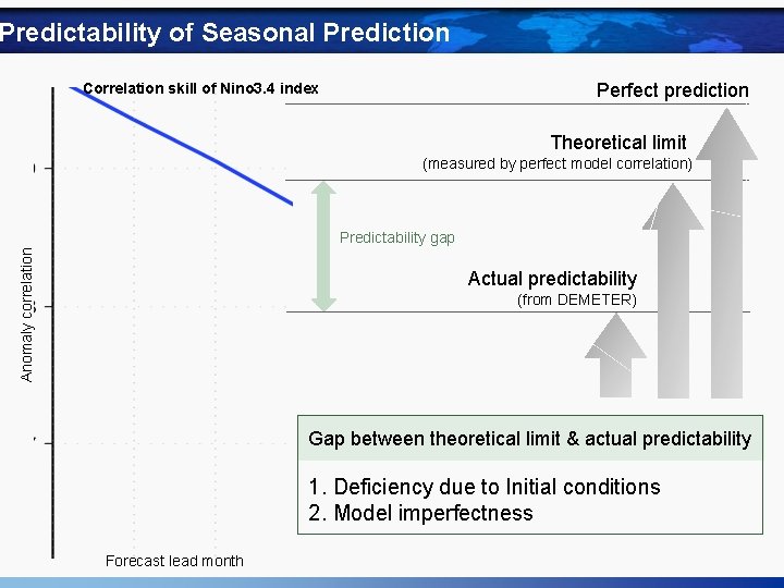
Predictability of Seasonal Prediction Perfect prediction Correlation skill of Nino 3. 4 index Theoretical limit (measured by perfect model correlation) Anomaly correlation Predictability gap Actual predictability (from DEMETER) Gap between theoretical limit & actual predictability 1. Deficiency due to Initial conditions 2. Model imperfectness Forecast lead month

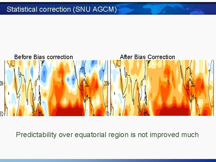
Statistical correction (SNU AGCM) Before Bias correction After Bias Correction Predictability over equatorial region is not improved much

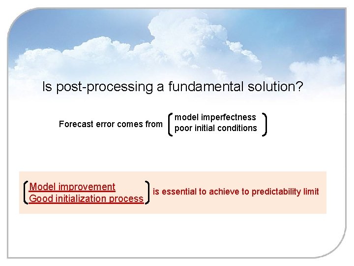
Is post-processing a fundamental solution? Forecast error comes from model imperfectness poor initial conditions Model improvement is essential to achieve to predictability limit Good initialization process

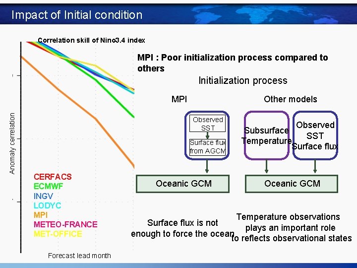
Impact of Initial condition Correlation skill of Nino 3. 4 index MPI : Poor initialization process compared to others Initialization process Anomaly correlation MPI Other models Observed SST Surface flux from AGCM CERFACS ECMWF INGV LODYC MPI METEO-FRANCE MET-OFFICE Forecast lead month Oceanic GCM Observed Subsurface SST Temperature Surface flux Oceanic GCM Temperature observations Surface flux is not plays an important role enough to force the ocean to reflects observational states

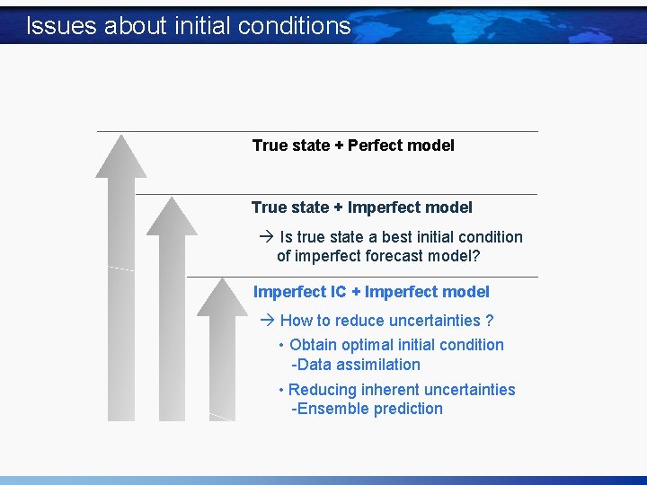
Issues about initial conditions True state + Perfect model True state + Imperfect model Is true state a best initial condition of imperfect forecast model? Imperfect IC + Imperfect model How to reduce uncertainties ? • Obtain optimal initial condition -Data assimilation • Reducing inherent uncertainties -Ensemble prediction

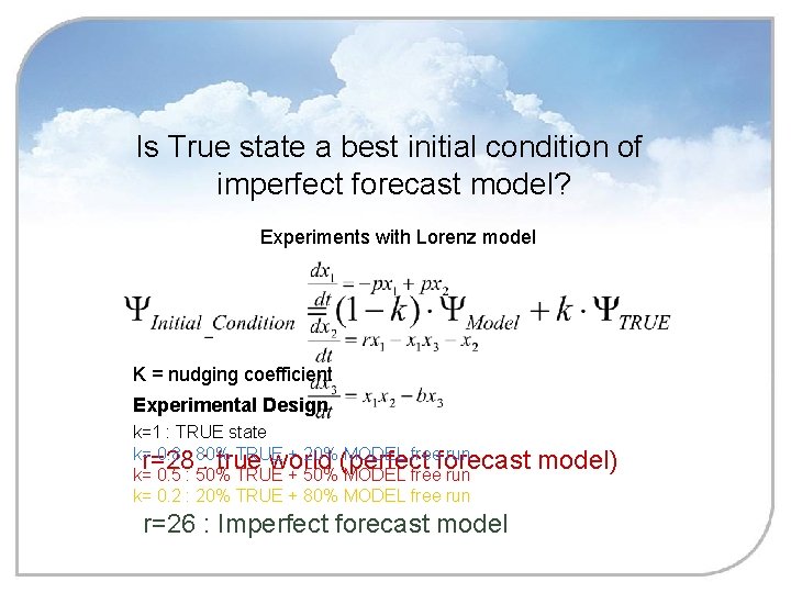
Is True state a best initial condition of imperfect forecast model? Experiments with Lorenz model K = nudging coefficient Experimental Design k=1 : TRUE state k= 0. 8 : 80% TRUE + 20% MODEL free run r=28 : true world (perfect forecast k= 0. 5 : 50% TRUE + 50% MODEL free run k= 0. 2 : 20% TRUE + 80% MODEL free run r=26 : Imperfect forecast model)

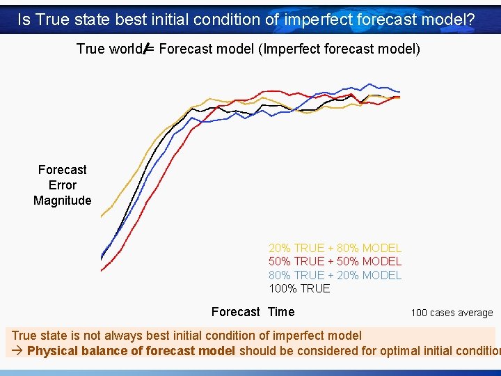
Is True state best initial condition of imperfect forecast model? True world = Forecast model (Imperfect forecast model) Forecast Error Magnitude 20% TRUE + 80% MODEL 50% TRUE + 50% MODEL 80% TRUE + 20% MODEL 100% TRUE Forecast Time 100 cases average True state is not always best initial condition of imperfect model Physical balance of forecast model should be considered for optimal initial condition

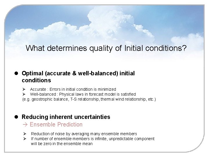
What determines quality of Initial conditions? l Optimal (accurate & well-balanced) initial conditions Ø Accurate : Errors in initial condition is minimized Ø Well-balanced : Physical laws in forecast model is satisfied (e. g. geostrophic balance, T-S relationship, thermal wind relationship, etc. ) l Reducing inherent uncertainties Ensemble Prediction Ø Ø Reduction of noise by averaging many ensemble members If number of ensemble members is infinite, unpredictable component will be zero in the ensemble mean

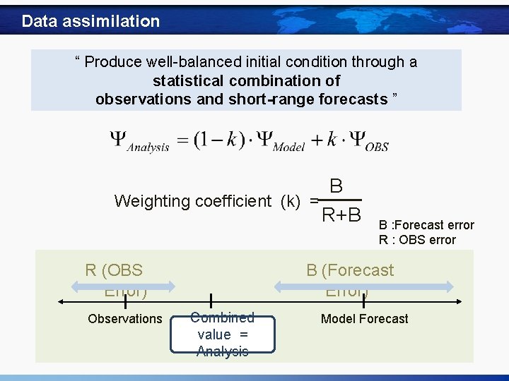
Data assimilation “ Produce well-balanced initial condition through a statistical combination of observations and short-range forecasts ” B Weighting coefficient (k) = R+B R (OBS Error) Observations B : Forecast error R : OBS error B (Forecast Error) Combined value = Analysis Model Forecast

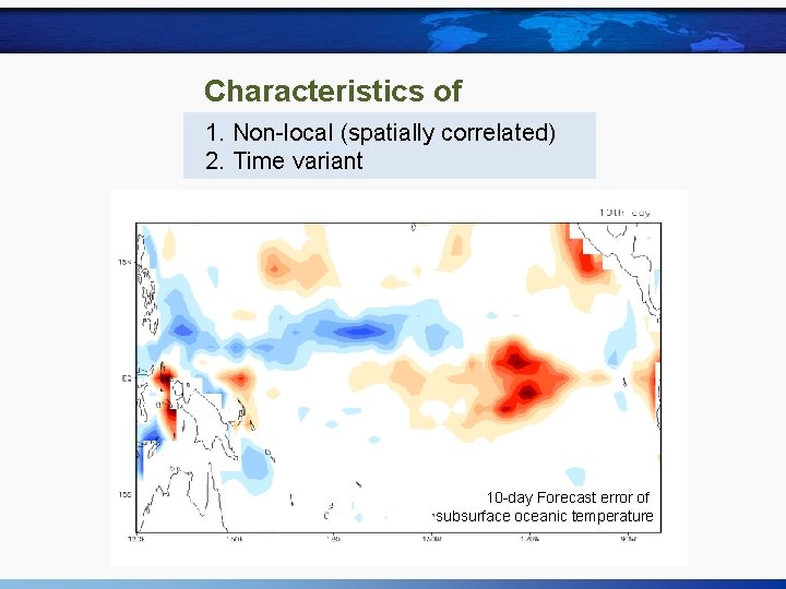
Characteristics of forecast 1. Non-localerror (spatially correlated) 2. Time variant 10 -day Forecast error of subsurface oceanic temperature

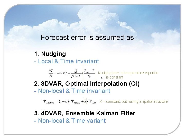
Forecast error is assumed as… 1. Nudging - Local & Time invariant Nudging term in temperature equation is constant 2. 3 DVAR, Optimal Interpolation (OI) - Non-local & Time invariant K = constant, but having a spatial structure 3. 4 DVAR, Ensemble Kalman Filter - Non-local & Time variant

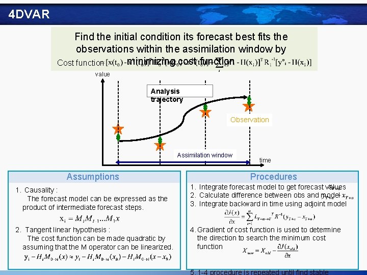
4 DVAR Find the initial condition its forecast best fits the observations within the assimilation window by minimizing cost function Cost function value Analysis trajectory Observation Assimilation window Assumptions time Procedures 1. Causality : The forecast model can be expressed as the product of intermediate forecast steps. 1. Integrate forecast model to get forecast values 2. Calculate difference between obs and model 3. Integrate backward in time using adjoint model 2. Tangent linear hypothesis : The cost function can be made quadratic by assuming that the M operator can be linearized. 4. Gradient of cost function is used to determine the direction to search the minimum cost function 5. 1 -4 procedure is repeated until find stable

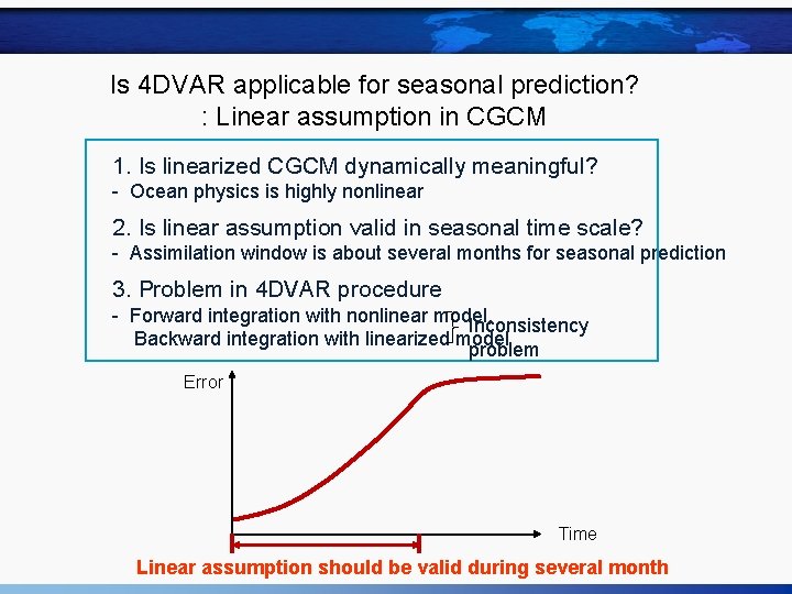
Is 4 DVAR applicable for seasonal prediction? : Linear assumption in CGCM 1. Is linearized CGCM dynamically meaningful? - Ocean physics is highly nonlinear 2. Is linear assumption valid in seasonal time scale? - Assimilation window is about several months for seasonal prediction 3. Problem in 4 DVAR procedure - Forward integration with nonlinear model, Inconsistency Backward integration with linearized model problem Error Time Linear assumption should be valid during several month

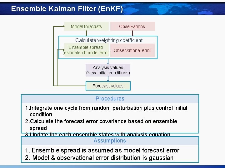
Ensemble Kalman Filter (En. KF) Model forecasts Observations Calculate weighting coefficient Ensemble spread (estimate of model error) Observational error Analysis values (New initial conditions) Forecast values Procedures 1. Integrate one cycle from random perturbation plus control initial condition 2. Calculate the forecast error covariance based on ensemble spread 3. Update the each ensemble states with analysis equation Assumptions 4. Repeat 1 -3 processes 1. Ensemble spread is assumed as model forecast error 2. Model & observational error distribution is gaussian

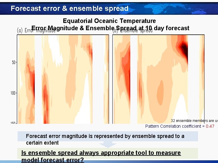
Forecast error & ensemble spread Equatorial Oceanic Temperature Error Magnitude & Ensemble Spread at 10 day forecast 32 ensemble members are us Pattern Correlation coefficient = 0. 47 Forecast error magnitude is represented by ensemble spread to a certain extent Is ensemble spread always appropriate tool to measure model forecast error?

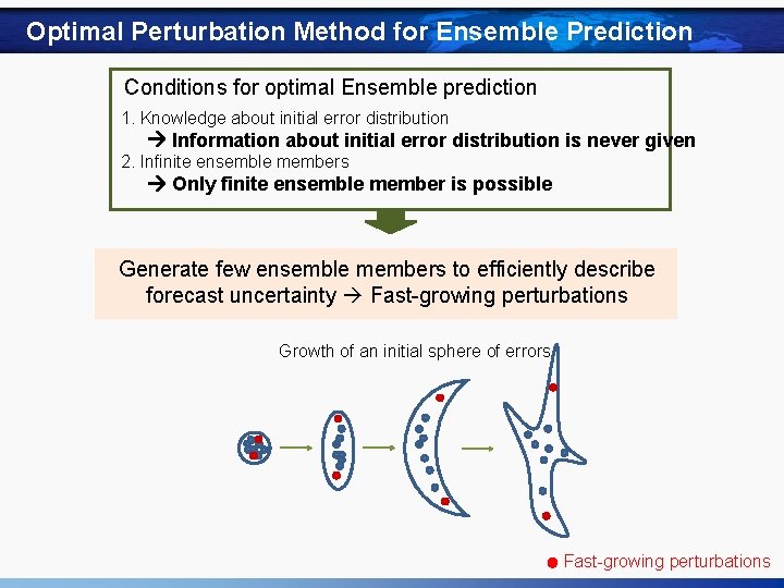
Optimal Perturbation Method for Ensemble Prediction Conditions for optimal Ensemble prediction 1. Knowledge about initial error distribution Information about initial error distribution is never given 2. Infinite ensemble members Only finite ensemble member is possible Generate few ensemble members to efficiently describe forecast uncertainty Fast-growing perturbations Growth of an initial sphere of errors Fast-growing perturbations

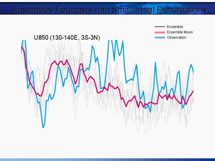
Ensembles Forecasts with Small Initial Perturbations U 850 (130 -140 E, 3 S-3 N) Ensemble Mean Observation

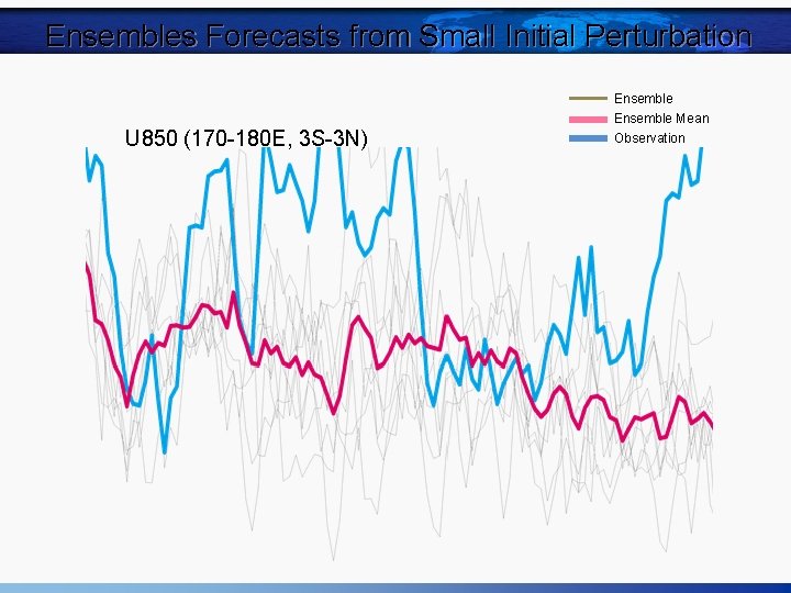
Ensembles Forecasts from Small Initial Perturbation U 850 (170 -180 E, 3 S-3 N) Ensemble Mean Observation

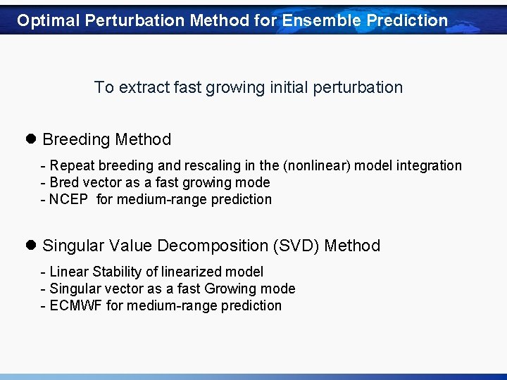
Optimal Perturbation Method for Ensemble Prediction To extract fast growing initial perturbation l Breeding Method - Repeat breeding and rescaling in the (nonlinear) model integration - Bred vector as a fast growing mode - NCEP for medium-range prediction l Singular Value Decomposition (SVD) Method - Linear Stability of linearized model - Singular vector as a fast Growing mode - ECMWF for medium-range prediction

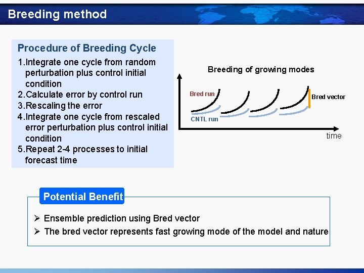
Breeding method Procedure of Breeding Cycle 1. Integrate one cycle from random perturbation plus control initial condition 2. Calculate error by control run 3. Rescaling the error 4. Integrate one cycle from rescaled error perturbation plus control initial condition 5. Repeat 2 -4 processes to initial forecast time Breeding of growing modes Bred run Bred vector CNTL run time Potential Benefit Ø Ensemble prediction using Bred vector Ø The bred vector represents fast growing mode of the model and nature

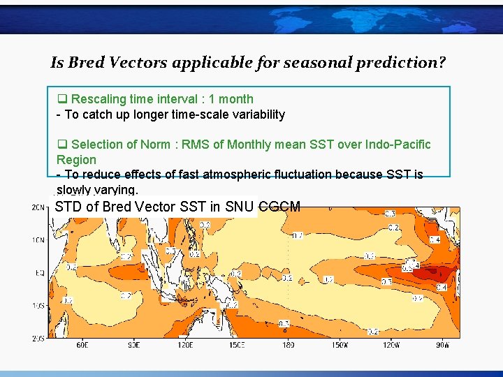
Is Bred Vectors applicable for seasonal prediction? q Rescaling time interval : 1 month - To catch up longer time-scale variability q Selection of Norm : RMS of Monthly mean SST over Indo-Pacific Region - To reduce effects of fast atmospheric fluctuation because SST is slowly varying. STD of Bred Vector SST in SNU CGCM

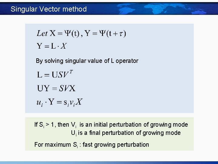
Singular Vector method By solving singular value of L operator If Si > 1, then Vi is an initial perturbation of growing mode Ui is a final perturbation of growing mode For maximum Si : fast growing perturbation

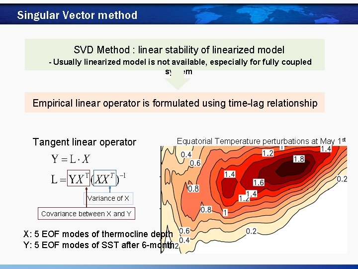
Singular Vector method SVD Method : linear stability of linearized model - Usually linearized model is not available, especially for fully coupled system Empirical linear operator is formulated using time-lag relationship Tangent linear operator Variance of X Covariance between X and Y X: 5 EOF modes of thermocline depth Y: 5 EOF modes of SST after 6 -month Equatorial Temperature perturbations at May 1 st

Thank you