Improved Ocean Initialization for Coupled Modelling for week2

Improved Ocean Initialization for Coupled Modelling for week-2 Monsoon forecast SUNEET DWIVEDI K Banerjee Centre of Atmospheric and Ocean Studies, M N Saha Centre of Space Studies University of Allahabad, INDIA

Objectives v Development, Configuration and Execution of Indian Ocean State Estimation system using Ocean component of Unified Model (UM) of Met Office (UK) and its associated Data Assimilation scheme (viz. NEMO and NEMOVAR) v Generation of quality controlled four-dimensional (threedimensional time varying) geophysical state of the Indian Ocean (with emphasis on ocean’s upper hydrographic/thermal structure and flow field) v To provide coherent estimates of space-time varying upper Ocean mixed layer depth

RELEVANCE q To achieve better prediction ability for medium-range monsoon forecast, improved Indian ocean initializations are important. q Observing the physical state of the Indian ocean is however challenging: size, high variability, lack of extant quality observations continuous in space and time. q Research expeditions are conducted to study specific processes at a regional scale, but such data suffers from being too sparse in space and time. q The satellite measurements have superior space/time coverage, but are they restricted to surface variables only, and can be hard to combine with in-situ data. q approach: use a ocean circulation model NEMO and optimally combine it with the available observations using NEMOVAR data assimilation

Outline (First Year Progress Report): v Indian Ocean circulation modeling around AS and Bo. B at 25 km resolution using NEMOAGRIF v Geophysical fields (3 -D time evolving flow field and hydrographic structure) of the region [70 -95 E; 0 -20 N] during 1996 -2007 (12 years) v Upper Ocean mixed layer depth variability

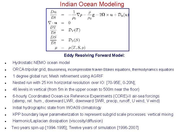
Indian Ocean Modeling Eddy Resolving Forward Model: Hydrostatic NEMO ocean model ORCA-tripolar grid, Boussinesq, incompressible Navier-Stokes equations, thermodynamics equations 1 degree global run; Mesh refinement using AGRIF Nested run with 25 Km horizontal resolution over IO: [70 -95 E, 0 -20 N]; 46 levels in vertical (from 5 m in the upper ocean to 500 m near the floor) 6 -hourly Coordinated Ocean-ice Reference Experiments (CORE)-II air-sea forcings (atemp, rel. hum. , downward LWR, downward SWR, precip, runoff, U wind, V wind) Initial hydrographic state from WOA 09 climatology KPP boundary layer parameterization to represent subgrid scale processes: vertical mixing Harmonic/Laplacian dissipation (viscosity/diffusion) Two years spin-up [1994 -1995]; Twelve years of simulation [1996 -2007]

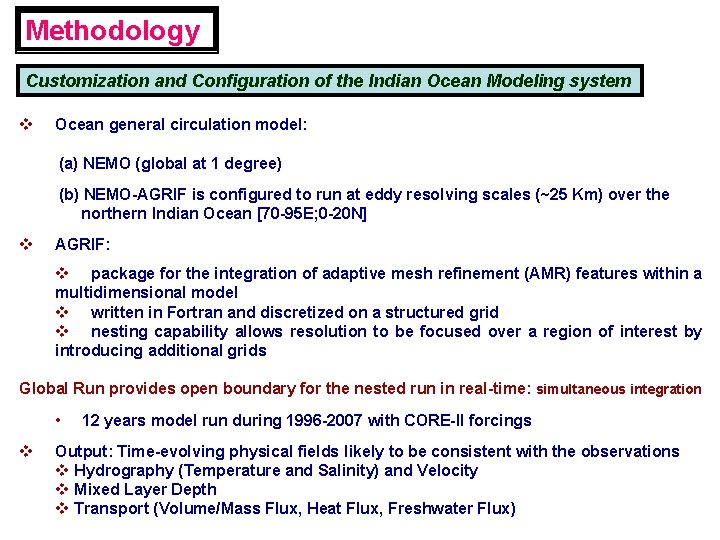
Methodology Customization and Configuration of the Indian Ocean Modeling system v Ocean general circulation model: (a) NEMO (global at 1 degree) (b) NEMO-AGRIF is configured to run at eddy resolving scales (~25 Km) over the northern Indian Ocean [70 -95 E; 0 -20 N] v AGRIF: v package for the integration of adaptive mesh refinement (AMR) features within a multidimensional model v written in Fortran and discretized on a structured grid v nesting capability allows resolution to be focused over a region of interest by introducing additional grids Global Run provides open boundary for the nested run in real-time: simultaneous integration • v 12 years model run during 1996 -2007 with CORE-II forcings Output: Time-evolving physical fields likely to be consistent with the observations v Hydrography (Temperature and Salinity) and Velocity v Mixed Layer Depth v Transport (Volume/Mass Flux, Heat Flux, Freshwater Flux)

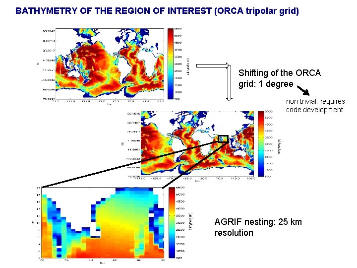
BATHYMETRY OF THE REGION OF INTEREST (ORCA tripolar grid) Shifting of the ORCA grid: 1 degree non-trivial: requires code development AGRIF nesting: 25 km resolution

Model: Monthly variability of the SST [1996: 2007] min during DJF in upper Bo. B; max during Apr-May

ORAS 4: Monthly variability of the SST [1996: 2007] • • Model is able to reasonably capture the monthly variability of the SST: r (model, ORAS 4) = 0. 96 Max SST bias is in the range of [-0. 3]o. C : higher near coastal regions; bias is nearly zero in most of the grid points SST mean square error between the model and ORAS 4 is 0. 3 o. C; smaller than the std dev (0. 9 o. C) of the SST

Model: Monthly variability of the SSS [1996: 2007]

ORAS 4: Monthly variability of the SSS [1996: 2007] • model underestimates the SSS: 2 -3 psu • incorrect mixing parametrization !!!!

Model: Monthly variability of the SSH [1996: 2007] Arabian sea SSH is very small compared to Bo. B throughout the year Bo. B: minimum SSH close to coast is during Aug-Oct; highest during Apr-May SSH becomes as high as 50 -60 cm in upper Bay and even higher near equator

ORAS 4: Monthly variability of the SSH [1996: 2007] • • Model SSH is underestimated in the Bo. B compared to ORAS 4 Bias is small compared to in GODAS, however

Model: Monthly variability of the MLD [1996: 2007] Ø lowest in the months of Mar-Apr-May; dipole like structure (jan and jul, for example) Ø post-monsoon months: intermediate values as a result of increased freshwater flux; increased wind speed and lower shortwave radiation

ORAS 4: Monthly variability of the MLD [1996: 2007]

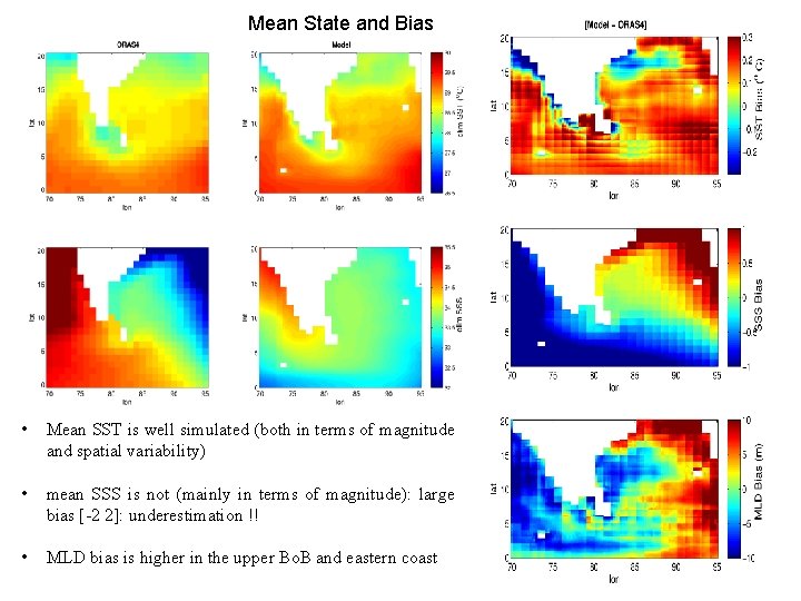
Mean State and Bias • Mean SST is well simulated (both in terms of magnitude and spatial variability) • mean SSS is not (mainly in terms of magnitude): large bias [-2 2]: underestimation !! • MLD bias is higher in the upper Bo. B and eastern coast

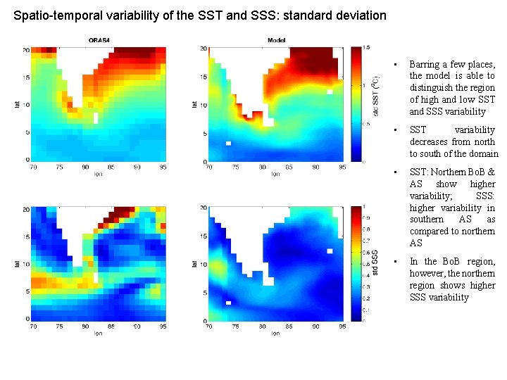
Spatio-temporal variability of the SST and SSS: standard deviation • Barring a few places, the model is able to distinguish the region of high and low SST and SSS variability • SST variability decreases from north to south of the domain • SST: Northern Bo. B & AS show higher variability; SSS: higher variability in southern AS as compared to northern AS • In the Bo. B region, however, the northern region shows higher SSS variability

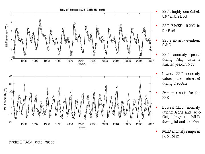
circle: ORAS 4; dots: model § SST : highly correlated: 0. 97 in the Bo. B § SST RMSE: 0. 2 o. C in the Bo. B § SST standard deviation: 0. 8 o. C § SST anomaly peaks during May with a smaller peak in Nov § lowest SST anomaly values are observed during Dec-Jan § Similar results for the SSS § Lowest MLD anomaly during April and Sept. Oct; highest MLD during Jul and Jan-Feb § MLD anomaly ranges in [-15 15] m

Model mean current is also well simulated fluxes will be computed ORAS 4

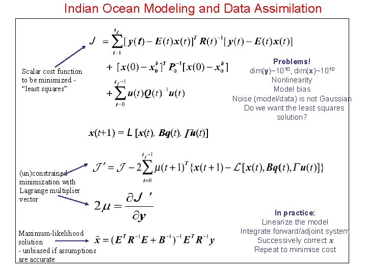
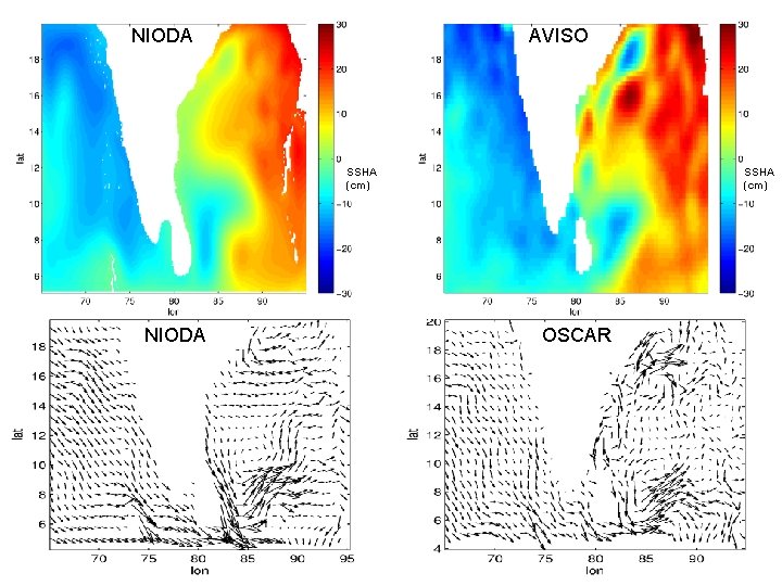
Future Work: High-resolution regional data assimilation using 4 D-Var Familiar Task: Customization, Configuration and Development of Ocean Data Assimilation system in the IO at a resolution of 10 km • ECCO and MITgcm groups have developed tools that produce state estimates using the 4 D-Var assimilation technique. • Remotely Sensed observations of SST, SSS and SSH and in-situ data of T, S are combined with the MITgcm (with realistic physics) using 4 D-Var for a period of 61 days [Jun-Jul 2013] • This method generates time-evolving fields that are statistically consistent with the observations, while obeying the model dynamics • It uses iterative procedure, which repeatedly integrates forward and adjoint model to minimize discrepancy between model and data Adjoint Model / Data Assimilation: Adjoint code using TAF Unconstrained minimization/Lagrange Multiplier Obs: SSH (AVISO), SST(GHRSST-OSTIA), SSS (Aquarius), T/S (ARGO) Optimization (successive iteration) to minimize (least-square) objective/cost function (model-data misfit)

Indian Ocean Modeling and Data Assimilation Problems! dim(y)~1010, dim(x)~1010 Nonlinearity Model bias Noise (model/data) is not Gaussian Do we want the least squares solution? Scalar cost function to be minimized “least squares” x(t+1) = L [x(t), Bq(t), u(t)] (un)constrained minimization with Lagrange multiplier vector Maximum-likelihood solution - unbiased if assumptions are accurate In practice: Linearize the model Integrate forward/adjoint system Successively correct x Repeat to minimise cost

NIODA GODAS ORAS 4

NIODA AVISO SSHA (cm) NIODA SSHA (cm) OSCAR

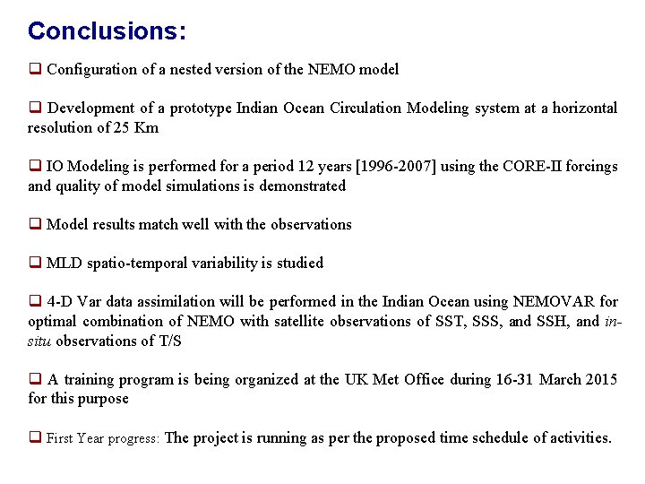
Conclusions: q Configuration of a nested version of the NEMO model q Development of a prototype Indian Ocean Circulation Modeling system at a horizontal resolution of 25 Km q IO Modeling is performed for a period 12 years [1996 -2007] using the CORE-II forcings and quality of model simulations is demonstrated q Model results match well with the observations q MLD spatio-temporal variability is studied q 4 -D Var data assimilation will be performed in the Indian Ocean using NEMOVAR for optimal combination of NEMO with satellite observations of SST, SSS, and SSH, and insitu observations of T/S q A training program is being organized at the UK Met Office during 16 -31 March 2015 for this purpose q First Year progress: The project is running as per the proposed time schedule of activities.

THANK YOU FOR YOUR PATIENCE