Damped Forced Oscillations Coupled Oscillations 1 The solution

Damped Forced Oscillations Coupled Oscillations 1

The solution for x in the equation of motion of a damped simple harmonic oscillator driven by an external force consists of two terms: a transient term (‘=temporary’) and a steady-state term 2

Transient Term The transient term dies away with time and is the solution to the equation discussed earlier: This contributes the term: x = Cept which decays with time as e-βt Steady-state Term The steady state term describes the behaviour of the oscillator after the transient term has died away. 3

Both terms contribute to the solution initially, but the ultimate behaviour of the oscillator is described by the ‘steady-state term’. Solutions Complementary Functions are transients It always dies out if there is damping. As a practical matter, it often suffices to know the particular solution. Steady State behaviour is decided by the Particular Integral 4

Driven Damped Oscillations: Transient and Steady-state behaviours 5 http: //comp. uark. edu/~mattclay/Teaching/Spring 2013/driven-motion. html

Forced oscillator: Damped case Time dependent function 6

Companion equation: General equation 7

Complementary function: Transients Try steady-state solution (Particular solution) 8

Try steady-state solution (Particular solution) (look at the flow of thought…) Consider a general sinusoidal drive force: Equation of motion becomes: The above equation is the real part of simplest complex differential equation: with x = Re(z) 9

Guess a solution based on physical and mathematical intuition. It is not obvious whether the angular frequency of this motion would be that of: - Oscillation without damping or driving ( o) - Oscillation with damping, but no driving ( ’) - Drive frequency ( ) - Or some combination of these? For now, we write the angular frequency of motion in steady state as s. A general guess would be: Plug into the equation: And obtain: 10

The left side oscillates at s, while the right side oscillated at . So, if they are to be equal, we must have s= . i. e. , In the steady-state, the oscillator moves with the same angular frequency as the drive force. So, our guess now becomes: Now, solving the equation gives: REAL: IMAGINARY: 11

REAL: IMAGINARY: To isolate |zo|, square these 2 equations and add them to give: To isolate , divide the above 2 equations: Our guess is the solution, if |zo| and are given as above. Then, the real part of the solution is: 12

Writing the amplitude in a different form It may appear that the max amplitude appears at = o. However, the term is multiplied by the factor 1/ , which increase as decreases, shifting the peak to a slightly lower value of o. This point of maximum amplitude is the resonance. We see that the response amplitude at high frequencies approaches zero. In the opposite limit We also see that the phase by which the oscillator’s response lags behind the drive force also depends on . When = o, then So that 13

Amplitude: Forced Damped Osc. -2 14

Show amplitude resonance at: 15

Amplitude Resonance At ω = ω0 16

Amplitude: The low and high frequency behaviour are the same as the situation without damping. The changes due to damping are in the vicinity of = o. Amplitude is finite throughout. The amplitude is maximum at:

Phase: The phase by which the oscillator’s response lags behind the drive force also depends on . When = o, then So that 18

19

For mild damping (β << o), = o (approximately). 20

21

Forced oscillations for different resistances In the case of larger resistance, the transients die faster. 22

Amplitude and phase 23

Different driving amplitudes In the case of larger forcing amplitude, steady state is reached quicker. 24

Compare with F(t) = F 0 cos ωt The motion of the oscillator is v independent of mass or damping. v stiffness controlled. v in phase with external force. 25

The motion of the oscillator is v independent of stiffness or damping. v mass controlled. v out of phase with external force. 26

The motion of the oscillator is v independent of mass or stiffness. v damping controlled. v of phase lag with external force. 27

High frequency and low frequency behaviour unchanged by damping Amplitude is finite throughout Summary Amplitude and Phase Resonance Mass-controlled Stiffness. Controlled Maximum Amplitude @ : Resonance 28

Velocity Resonance Show that velocity resonance frequency ωvres= ω0 and velocity resonance amplitude

Instantaneous power absorbed by the system: (Power drawn by the oscillator from the external force) Average power over one cycle: 30

We know:

Peak Power: 8 2 Maximum average power is absorbed at resonance Using this it can be shown that: Width at half peak power (FWHM) = 2, 1 From here one can measure the damping parameter: r 32

Average power absorbed = < P > Lorentzian Profile - Seen in situations where we have a resonance - Has a peak at = o /2 = 3 ω1 ω2 ω0 33

Resonant quality factor: = Central frequency FWHM Quantifies the sharpness of resonance curves. 34

Stored energy: Problem: What is the peak value and at what driving frequency? 35

Stored energy: < E > = 3 36

Resonance (Interesting Examples) 37

If you push a person on a swing, you must put the energy in at just the natural frequency of the swing or some multiple of it. The motion will build up in amplitude to the point where it is limited by the damping forces on the system. If the damping forces are small, a resonant system can build up to amplitudes large enough to be destructive to the system. - Using Resonance to shatter a Kidney stone: By tuning ultra sound waves to the natural frequency of a kidney stone, we can rely on resonance to pulverize the stone. - MRI http: //www. regentsprep. org/regents/physics/phys 04/bresonan/default. htm 38

Angers Bridge over river Maine in France Angers Bridge was a suspension bridge over the Maine River in Angers, France. The bridge collapsed when 478 French soldiers marched across it in lockstep. Since the soldiers were marching together, they caused the bridge to vibrate and twist from side to side, dislodging an anchoring cable from its concrete mooring. Though a storm also raged during the collapse, engineering experts indicate the collapse was due to the soldiers instead of the storm. Collapsed under weight of marching troops, April 16, 1850, killing more than 200 soldiers. 39

Millennium Bridge, London When the Millennium Bridge was opened in 2000, the motion of pedestrians caused it to vibrate, and they fell into step with the vibrations, increasing them. The problem at the Millennium Bridge was corrected during the next two years. Soldiers break step while crossing bridges. http: //en. wikipedia. org/wiki/Millennium_Bridge_%28 London%29#Resonance 40

Tacoma Narrows Bridge The Tacoma Narrows Bridge is a mile-long (1600 meter) suspension bridge with a main span of 850 m (the third-largest in the world when it was first built) that carried Washington State Route 16 across the Tacoma Narrows of Puget Sound from Tacoma to Gig Harbor, Washington (collapsed in wind, 1940) http: //www. enm. bris. ac. uk/anm/tacoma. html 41

Coupled Oscillations 42

Coupled oscillations Waves 43

Coupled oscillators 44

Coupled pendula θo θ 1 l xo Mass-0 k x 1 Mass-1 45

Forces acting on a Simple oscillators 46

Considering small-angle approximation Equation of motion θo θ 1 l xo Mass-0 k x 1 Total force on Mass-0 Mass-1 SHM term Coupling term 47

Let Natural freq. of each pendulum Adding Subtracting 48

These are coupled differential equations. We have to identify linear combinations of x 0 and x 1 for which the equations become decoupled. In this case, we can easily identify 2 such variables (q 1 and q 2): 49

Normal Co-ordinates Normal modes Normal coordinates are coordinates in which the equations of motion take the form of a set of linear differential equations with constant coefficients in which each equation contains only one dependent variable. (Here, simple harmonic equations are in q 1 and q 2 only) A vibration involving only one dependent variable is called a normal mode of vibration and has its own normal frequency. The importance of the normal modes of vibration is that they are entirely independent of each other. The energy associated with a normal mode is never exchanged with another mode; this is why we can add the energies of the separate modes to give the total energy.

Normal mode: A way in which the system can move in a steady state, in which all parts of the system move with the same frequency. The parts may have different (zero or negative) amplitudes. Breathing mode C-H Bending mode C-C Stretching mode 51

Normal modes of Vibration of molecule http: //chemwiki. ucdavis. edu/Physical_Chemistry/Spectroscopy/Vibrational_Modes 52

Normal frequencies Slow mode Fast mode 53

Normal mode amplitudes : q 10 and q 20 54

In-phase vibration (Pendulum mode) 55

Out-of-phase vibration (Breathing mode) 56

Coupled Oscillations To simplify discussion, let us choose: Initial conditions 57

Pendulum displacements 58

Behavior with time for individual pendulum 59

Condition for complete energy exchange The masses, M 0 and M 1, have to be equal. And, For xo=0 Else, neither of the two pendulums will ever be stationary 60

61

Resonance q 1 + q 2 62

Normal mode frequencies 63

64

Stiff coupling Slow oscillation will be missing 65

Coupled oscillators 66

Equations of motion 67

Normal modes The two normal modes execute SHO with respective angular frequencies 68

Normal modes: Physical Interpretation qo represents Centre of mass Slow mode 69

q 1 represents Relative coordinate (relative motion of the two masses with the centre of mass unchanged) Fast mode 70

71

72

The normal modes have solutions 73

74

i. e. , |Ao| sin ψ = 0 which gives initial phase ψ = 0 Remember 75

Resonance + 76

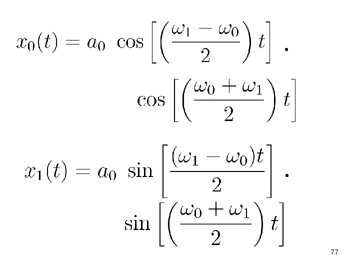
T B/ 2 TB=Beats Period x 0 (t) t TC Coupled oscillations (Resonance) x 1 (t) t 78

k’<< k 79

k’ >> k Connecting two masses with rigid rod 80