Image Alignment and Mosaicing Image Alignment Applications Local

Image Alignment and Mosaicing

Image Alignment Applications • Local alignment: – Tracking – Stereo • Global alignment: – Camera jitter elimination – Image enhancement – Panoramic mosaicing

Image Stitching Problems • Motion model • Parameterization • Correspondence • Warping • Blending

Motion Model • How do images relate to each other? • Possibilities: – Pure translation – Rigid body (translation + rotation) – Affine – Parallax – General motion

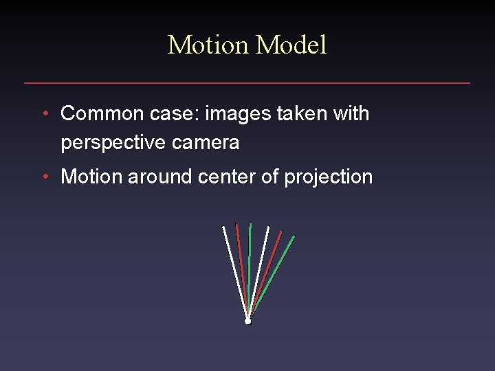
Motion Model • Common case: images taken with perspective camera • Motion around center of projection

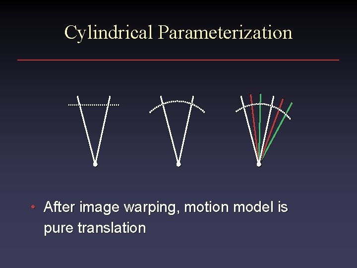
Parameterization • Single parameterization for all images • Cylindrical parameterization often used for panoramic mosaics

Cylindrical Parameterization • After image warping, motion model is pure translation

Correspondence Approaches • Optical flow • Correlation + optical flow • Any of the above, iterated (e. g. Lucas. Kanade) • Any of the above, coarse-to-fine

Correspondence Approaches • Optical flow • Correlation + optical flow • Any of the above, iterated (e. g. Lucas. Kanade) • Any of the above, coarse-to-fine

Optical Flow for Image Registration • Compute local matches • Least-squares fit to motion model • Problem: outliers

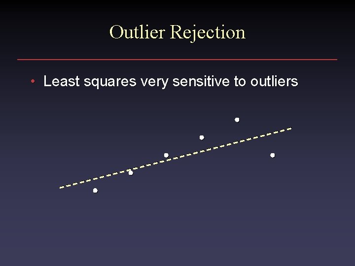
Outlier Rejection • Least squares very sensitive to outliers

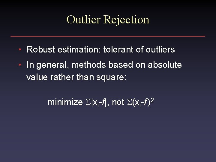
Outlier Rejection • Robust estimation: tolerant of outliers • In general, methods based on absolute value rather than square: minimize S|xi-f|, not S(xi-f )2

Robust Fitting • In general, hard to compute • Analytic solutions in a few cases – Mean Median – Solution for fitting lines

Approximation to Robust Fitting • Compute least squares • Assign weights based on average deviation – Simplest: weight = 1 if deviation < 2. 5 s, 0 otherwise – Smoother version: weight = Gs (deviation) • Weighted least squares • Iterate

Alternative Approximation to Robust Fitting • Least median of squares: – Select n random subsets of data points – Perform least-squares fit on each – Compute average deviation for each – Select fit with median deviation

Correspondence Approaches • Optical flow • Correlation + optical flow • Any of the above, iterated (e. g. Lucas. Kanade) • Any of the above, coarse-to-fine

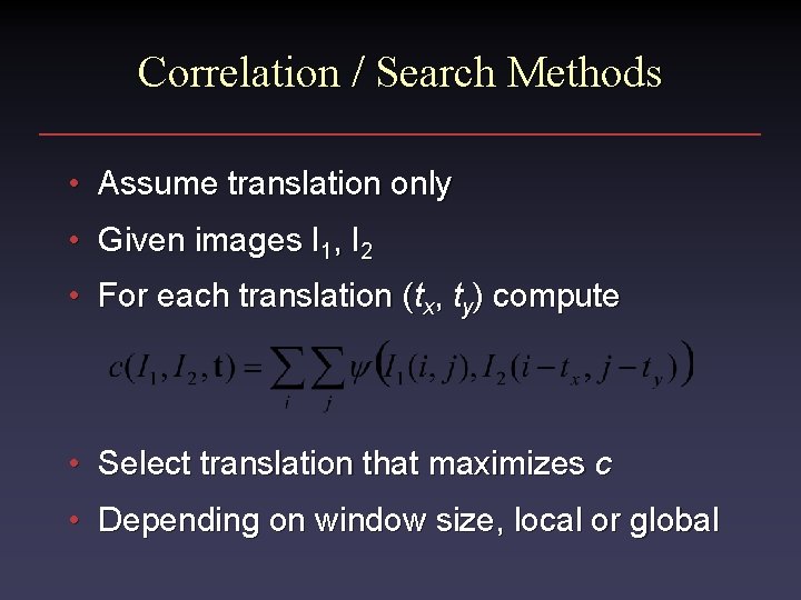
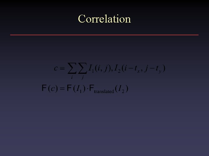
Correlation / Search Methods • Assume translation only • Given images I 1, I 2 • For each translation (tx, ty) compute • Select translation that maximizes c • Depending on window size, local or global

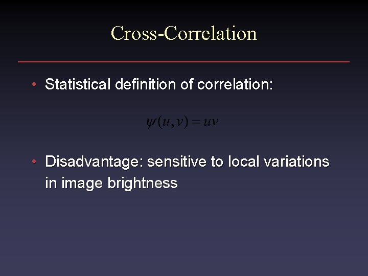
Cross-Correlation • Statistical definition of correlation: • Disadvantage: sensitive to local variations in image brightness

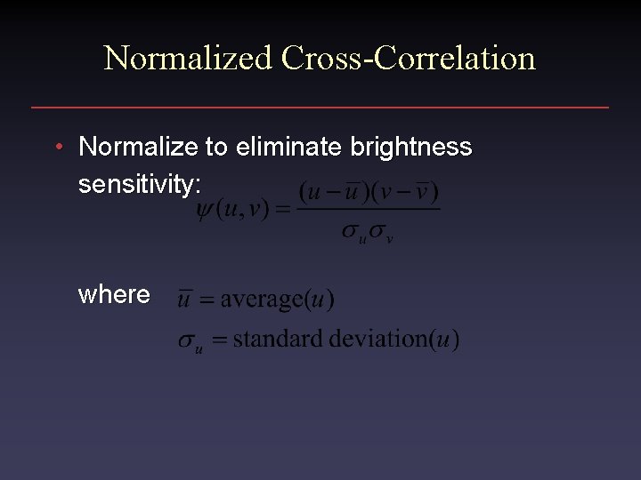
Normalized Cross-Correlation • Normalize to eliminate brightness sensitivity: where

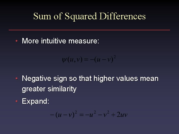
Sum of Squared Differences • More intuitive measure: • Negative sign so that higher values mean greater similarity • Expand:

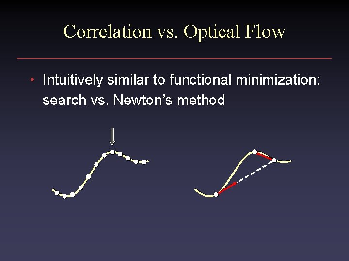
Correlation vs. Optical Flow • Intuitively similar to functional minimization: search vs. Newton’s method

Local vs. Global • Correlation with local windows not too expensive • High cost if window size = whole image • But computation looks like convolution – FFT to the rescue!

Correlation

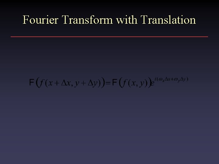
Fourier Transform with Translation

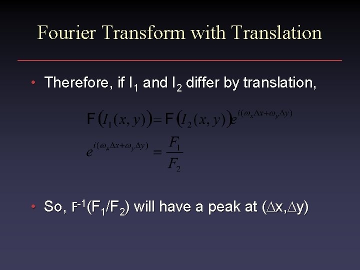
Fourier Transform with Translation • Therefore, if I 1 and I 2 differ by translation, • So, F-1(F 1/F 2) will have a peak at (Dx, Dy)

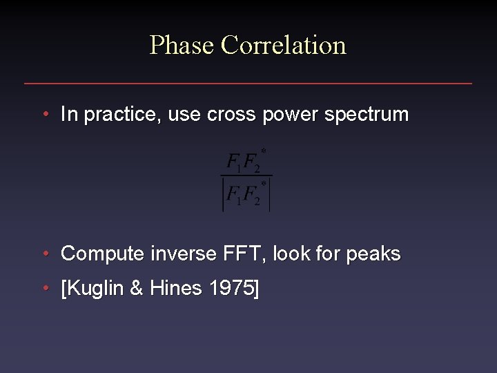
Phase Correlation • In practice, use cross power spectrum • Compute inverse FFT, look for peaks • [Kuglin & Hines 1975]

Phase Correlation • Advantages – Fast computation – Low sensitivity to global brightness changes (since equally sensitive to all frequencies)

Phase Correlation • Disadvantages – Sensitive to white noise – No robust version – Translation only • • • Extensions to rotation, scale But not local motion Not too bad in practice with small local motions

Correspondence Approaches • Optical flow • Correlation + optical flow • Any of the above, iterated (e. g. Lucas. Kanade) • Any of the above, coarse-to-fine

Correlation plus Optical Flow • Use e. g. phase correlation to find average translation (may be large) • Use optical flow to find local motions

Correspondence Approaches • Optical flow • Correlation + optical flow • Any of the above, iterated (e. g. Lucas. Kanade) • Any of the above, coarse-to-fine

Iteration • Local refinement of optical flow estimate • Sort of equivalent to multiple iterations of Newton’s method

Correspondence Approaches • Optical flow • Correlation + optical flow • Any of the above, iterated (e. g. Lucas. Kanade) • Any of the above, coarse-to-fine

Image Pyramids • Pre-filter images to collect information at different scales • More efficient computation, allows larger motions

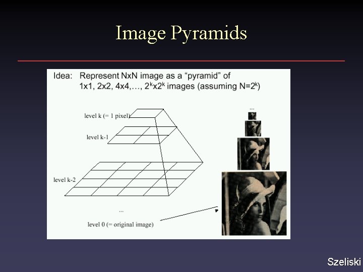
Image Pyramids Szeliski

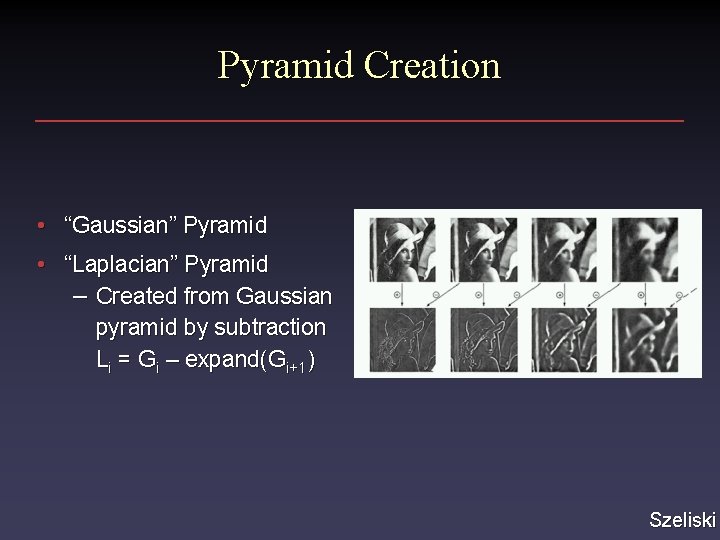
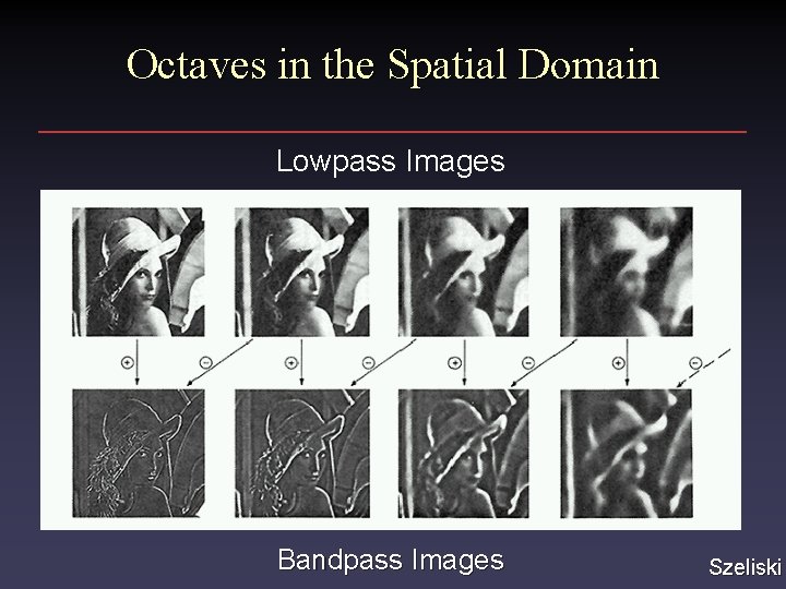
Pyramid Creation • “Gaussian” Pyramid • “Laplacian” Pyramid – Created from Gaussian pyramid by subtraction Li = Gi – expand(Gi+1) Szeliski

Octaves in the Spatial Domain Lowpass Images Bandpass Images Szeliski

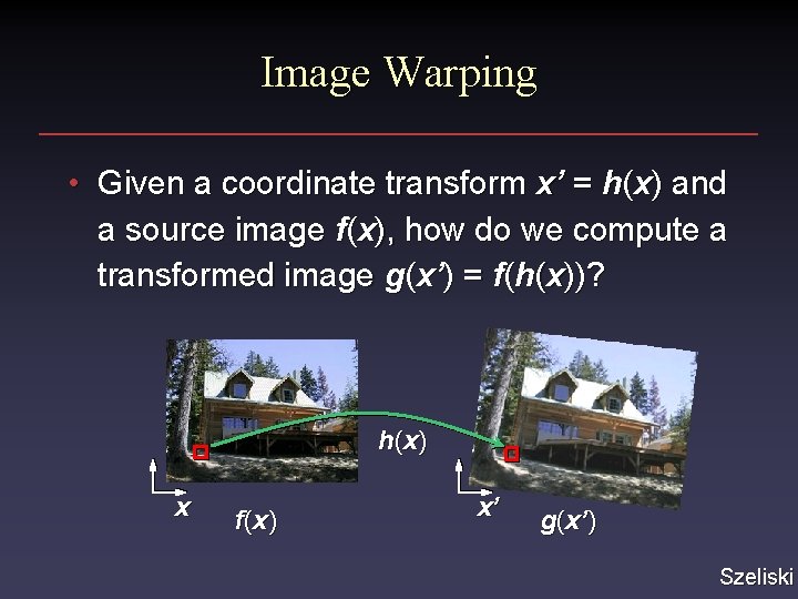
Image Warping • Given a coordinate transform x’ = h(x) and a source image f(x), how do we compute a transformed image g(x’) = f(h(x))? h (x ) x f(x ) x’ g(x’) Szeliski

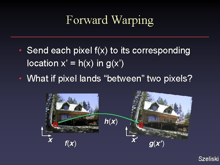
Forward Warping • Send each pixel f(x) to its corresponding location x’ = h(x) in g(x’) • What if pixel lands “between” two pixels? h (x ) x f(x ) x’ g(x’) Szeliski

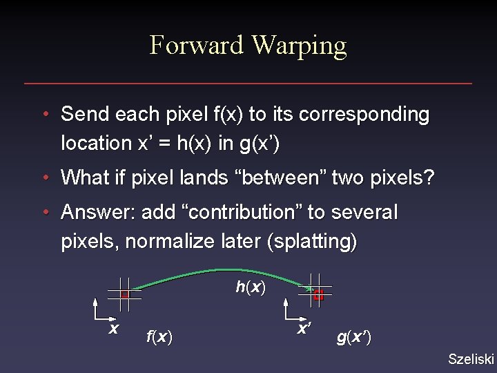
Forward Warping • Send each pixel f(x) to its corresponding location x’ = h(x) in g(x’) • What if pixel lands “between” two pixels? • Answer: add “contribution” to several pixels, normalize later (splatting) h (x ) x f(x ) x’ g(x’) Szeliski

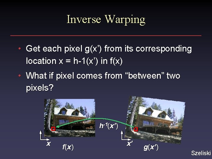
Inverse Warping • Get each pixel g(x’) from its corresponding location x = h-1(x’) in f(x) • What if pixel comes from “between” two pixels? h-1(x’) x f(x ) x’ g(x’) Szeliski

Inverse Warping • Get each pixel g(x’) from its corresponding location x = h-1(x’) in f(x) • What if pixel comes from “between” two pixels? • Answer: resample color value from interpolated (prefiltered) source image Szeliski

Blending • Blend over too small a region: seams • Blend over too large a region: ghosting

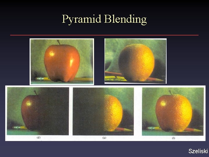
Multiresolution Blending • Different blending regions for different levels in a pyramid [Burt & Adelson] – Blend low frequencies over large regions (minimize seams due to brightness variations) – Blend high frequencies over small regions (minimize ghosting)

Pyramid Blending Szeliski

Minimum-Cost Cuts • Instead of blending high frequencies along a straight line, blend along line of minimum differences in image intensities

Minimum-Cost Cuts Moving object, simple blending blur [Davis 98]

Minimum-Cost Cuts Minimum-cost cut no blur [Davis 98]