Automatic Image Alignment direct with a lot of

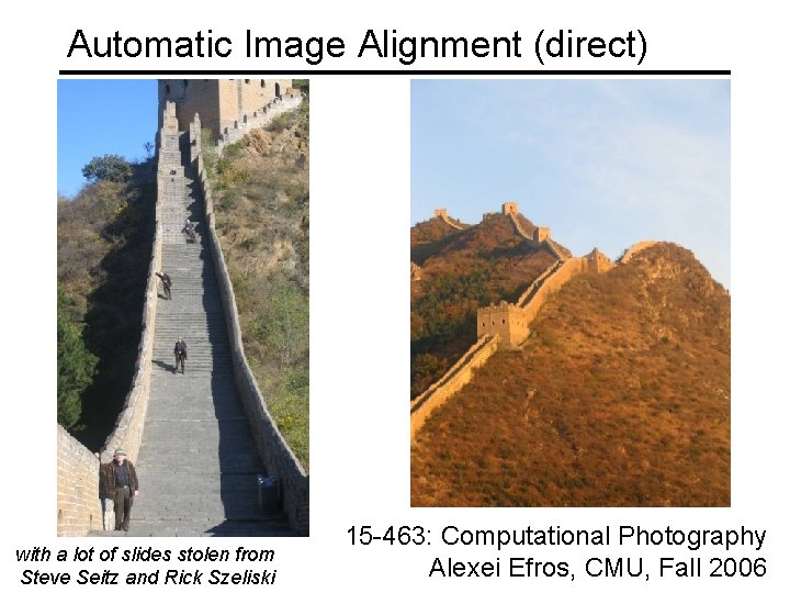
Automatic Image Alignment (direct) with a lot of slides stolen from Steve Seitz and Rick Szeliski 15 -463: Computational Photography Alexei Efros, CMU, Fall 2006

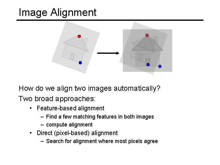
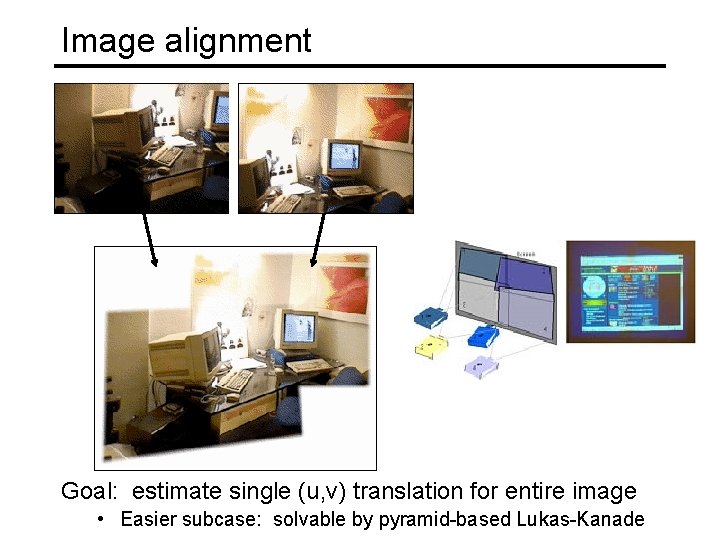
Image Alignment How do we align two images automatically? Two broad approaches: • Feature-based alignment – Find a few matching features in both images – compute alignment • Direct (pixel-based) alignment – Search for alignment where most pixels agree

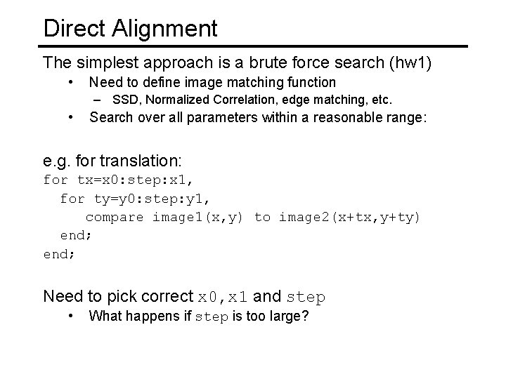
Direct Alignment The simplest approach is a brute force search (hw 1) • Need to define image matching function – SSD, Normalized Correlation, edge matching, etc. • Search over all parameters within a reasonable range: e. g. for translation: for tx=x 0: step: x 1, for ty=y 0: step: y 1, compare image 1(x, y) to image 2(x+tx, y+ty) end; Need to pick correct x 0, x 1 and step • What happens if step is too large?

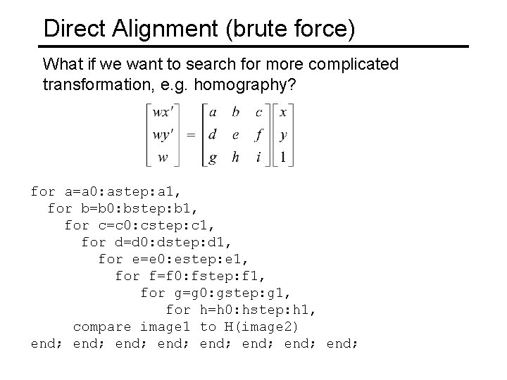
Direct Alignment (brute force) What if we want to search for more complicated transformation, e. g. homography? for a=a 0: astep: a 1, for b=b 0: bstep: b 1, for c=c 0: cstep: c 1, for d=d 0: dstep: d 1, for e=e 0: estep: e 1, for f=f 0: fstep: f 1, for g=g 0: gstep: g 1, for h=h 0: hstep: h 1, compare image 1 to H(image 2) end; end;

Problems with brute force Not realistic • Search in O(N 8) is problematic • Not clear how to set starting/stopping value and step What can we do? • Use pyramid search to limit starting/stopping/step values • For special cases (rotational panoramas), can reduce search slightly to O(N 4): – H = K 1 R 1 R 2 -1 K 2 -1 (4 DOF: f and rotation) Alternative: gradient decent on the error function • i. e. how do I tweak my current estimate to make the SSD error go down? • Can do sub-pixel accuracy • BIG assumption? – Images are already almost aligned (<2 pixels difference!) – Can improve with pyramid • Same tool as in motion estimation

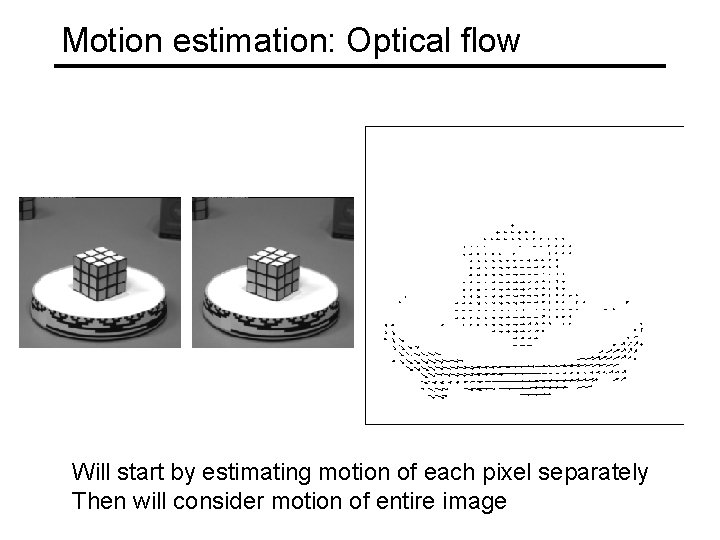
Motion estimation: Optical flow Will start by estimating motion of each pixel separately Then will consider motion of entire image

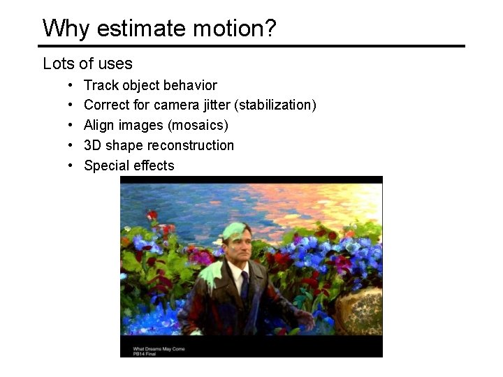
Why estimate motion? Lots of uses • • • Track object behavior Correct for camera jitter (stabilization) Align images (mosaics) 3 D shape reconstruction Special effects

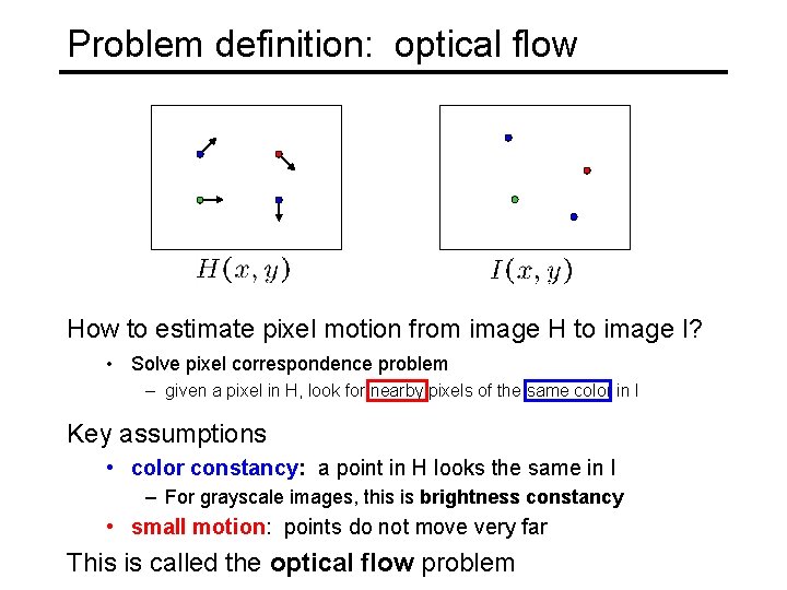
Problem definition: optical flow How to estimate pixel motion from image H to image I? • Solve pixel correspondence problem – given a pixel in H, look for nearby pixels of the same color in I Key assumptions • color constancy: a point in H looks the same in I – For grayscale images, this is brightness constancy • small motion: points do not move very far This is called the optical flow problem

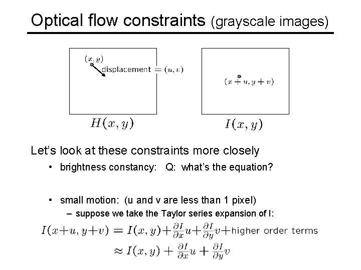
Optical flow constraints (grayscale images) Let’s look at these constraints more closely • brightness constancy: Q: what’s the equation? • small motion: (u and v are less than 1 pixel) – suppose we take the Taylor series expansion of I:

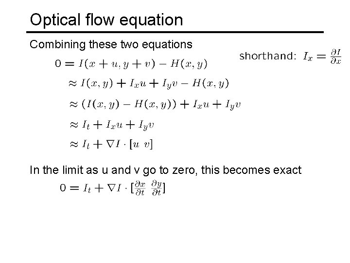
Optical flow equation Combining these two equations In the limit as u and v go to zero, this becomes exact

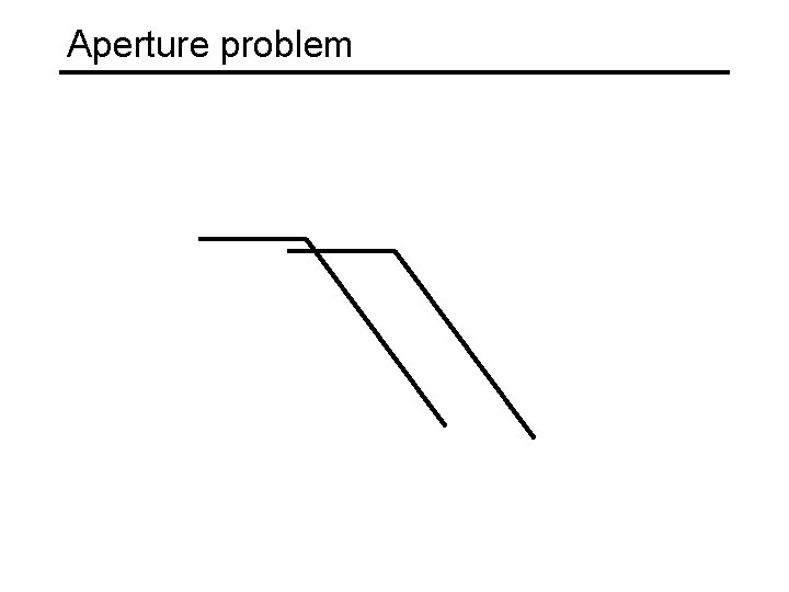
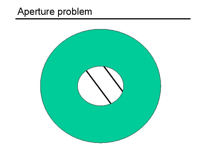
Optical flow equation Q: how many unknowns and equations per pixel? Intuitively, what does this constraint mean? • The component of the flow in the gradient direction is determined • The component of the flow parallel to an edge is unknown This explains the Barber Pole illusion http: //www. sandlotscience. com/Ambiguous/barberpole. htm

Aperture problem

Aperture problem

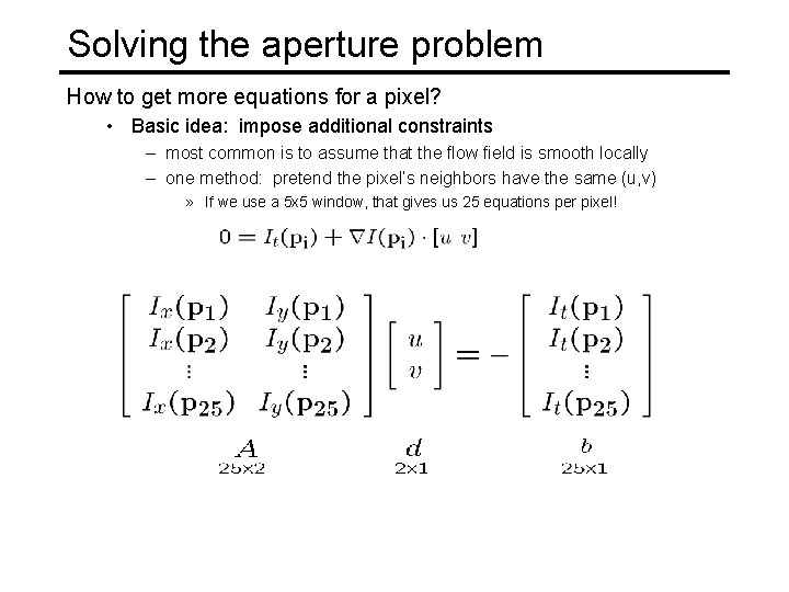
Solving the aperture problem How to get more equations for a pixel? • Basic idea: impose additional constraints – most common is to assume that the flow field is smooth locally – one method: pretend the pixel’s neighbors have the same (u, v) » If we use a 5 x 5 window, that gives us 25 equations per pixel!

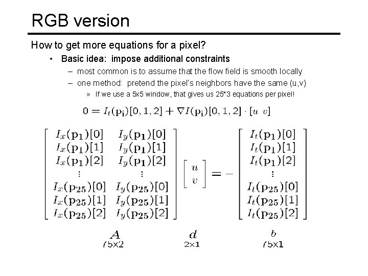
RGB version How to get more equations for a pixel? • Basic idea: impose additional constraints – most common is to assume that the flow field is smooth locally – one method: pretend the pixel’s neighbors have the same (u, v) » If we use a 5 x 5 window, that gives us 25*3 equations per pixel!

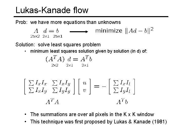
Lukas-Kanade flow Prob: we have more equations than unknowns Solution: solve least squares problem • minimum least squares solution given by solution (in d) of: • The summations are over all pixels in the K x K window • This technique was first proposed by Lukas & Kanade (1981)

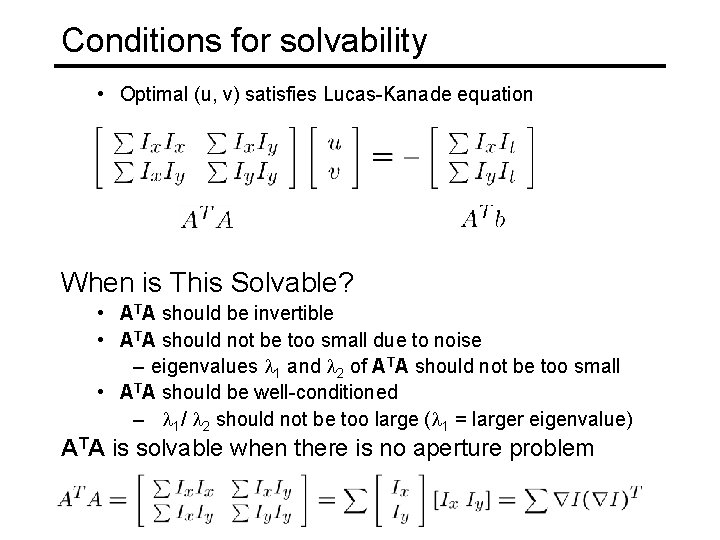
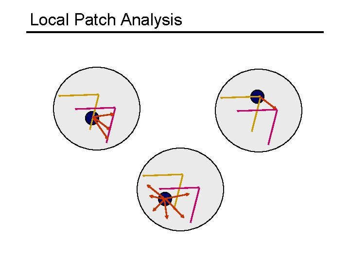
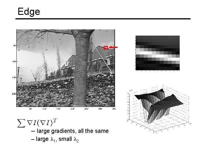
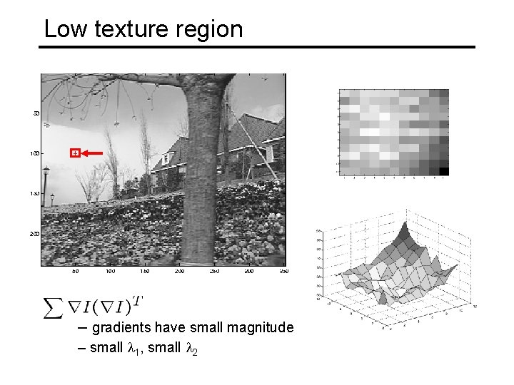
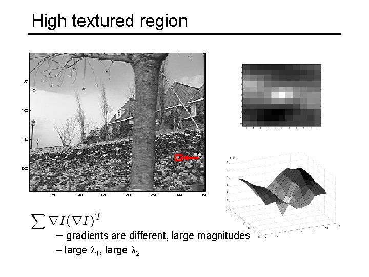
Conditions for solvability • Optimal (u, v) satisfies Lucas-Kanade equation When is This Solvable? • ATA should be invertible • ATA should not be too small due to noise – eigenvalues l 1 and l 2 of ATA should not be too small • ATA should be well-conditioned – l 1/ l 2 should not be too large (l 1 = larger eigenvalue) ATA is solvable when there is no aperture problem

Local Patch Analysis

Edge – large gradients, all the same – large l 1, small l 2

Low texture region – gradients have small magnitude – small l 1, small l 2

High textured region – gradients are different, large magnitudes – large l 1, large l 2

Observation This is a two image problem BUT • Can measure sensitivity by just looking at one of the images! • This tells us which pixels are easy to track, which are hard – very useful later on when we do feature tracking. . .

Errors in Lukas-Kanade What are the potential causes of errors in this procedure? • Suppose ATA is easily invertible • Suppose there is not much noise in the image When our assumptions are violated • Brightness constancy is not satisfied • The motion is not small • A point does not move like its neighbors – window size is too large – what is the ideal window size?

Iterative Refinement Iterative Lukas-Kanade Algorithm 1. Estimate velocity at each pixel by solving Lucas-Kanade equations 2. Warp H towards I using the estimated flow field - use image warping techniques 3. Repeat until convergence

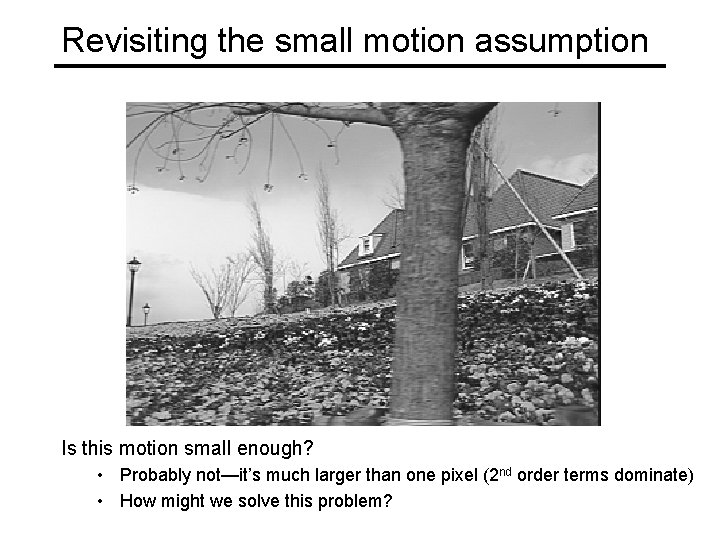
Revisiting the small motion assumption Is this motion small enough? • Probably not—it’s much larger than one pixel (2 nd order terms dominate) • How might we solve this problem?

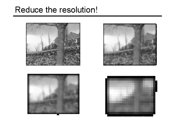
Reduce the resolution!

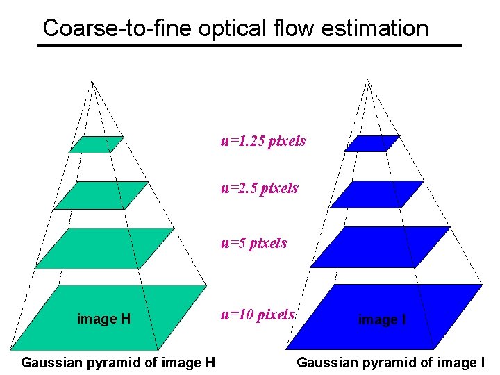
Coarse-to-fine optical flow estimation u=1. 25 pixels u=2. 5 pixels u=5 pixels image H Gaussian pyramid of image H u=10 pixels image II image Gaussian pyramid of image I

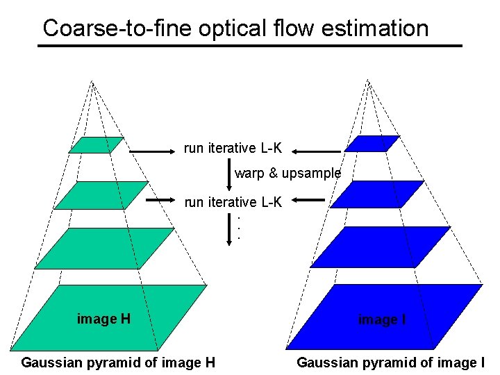
Coarse-to-fine optical flow estimation run iterative L-K warp & upsample run iterative L-K. . . image JH Gaussian pyramid of image H image II image Gaussian pyramid of image I

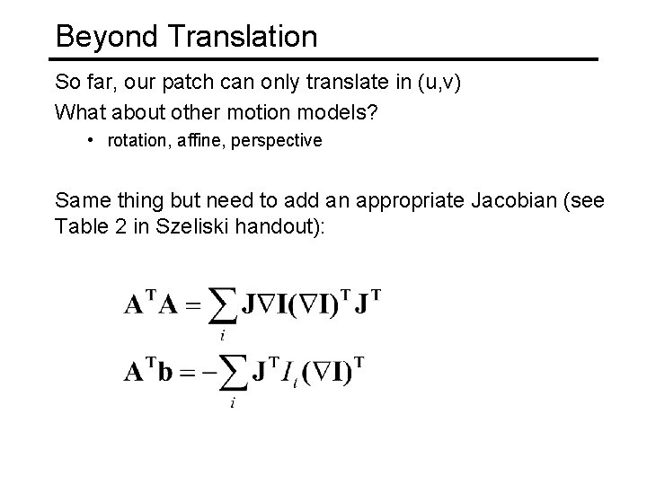
Beyond Translation So far, our patch can only translate in (u, v) What about other motion models? • rotation, affine, perspective Same thing but need to add an appropriate Jacobian (see Table 2 in Szeliski handout):

Image alignment Goal: estimate single (u, v) translation for entire image • Easier subcase: solvable by pyramid-based Lukas-Kanade

Lucas-Kanade for image alignment Pros: • All pixels get used in matching • Can get sub-pixel accuracy (important for good mosaicing!) • Relatively fast and simple Cons: • Prone to local minima • Images need to be already well-aligned What if, instead, we extract important “features” from the image and just align these?

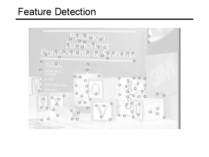
Feature-based alignment 1. Find a few important features (aka Interest Points) 2. Match them across two images 3. Compute image transformation as per Project #3 How do we choose good features? • • They must prominent in both images Easy to localize Think how you did that by hand in Project #3 Corners!

Feature Detection

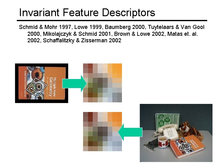
Feature Matching How do we match the features between the images? • Need a way to describe a region around each feature – e. g. image patch around each feature • Use successful matches to estimate homography – Need to do something to get rid of outliers Issues: • What if the image patches for several interest points look similar? – Make patch size bigger • What if the image patches for the same feature look different due to scale, rotation, etc. – Need an invariant descriptor

Invariant Feature Descriptors Schmid & Mohr 1997, Lowe 1999, Baumberg 2000, Tuytelaars & Van Gool 2000, Mikolajczyk & Schmid 2001, Brown & Lowe 2002, Matas et. al. 2002, Schaffalitzky & Zisserman 2002