HECRAS Introduction to Unsteady flow Jon Fripp NDCSMC

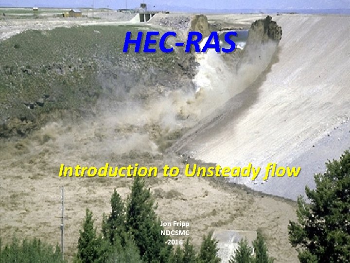
HEC-RAS Introduction to Unsteady flow Jon Fripp NDCSMC 2016

Module: 1 -D Unsteady Flow Introduction • Steady vs Unsteady • Why use unsteady flow • Introduction to 1 -D Unsteady HECRAS modeling – Data Input • Geometry • Boundary conditions • Flow – Calibration • Run a Unsteady file • View the Output

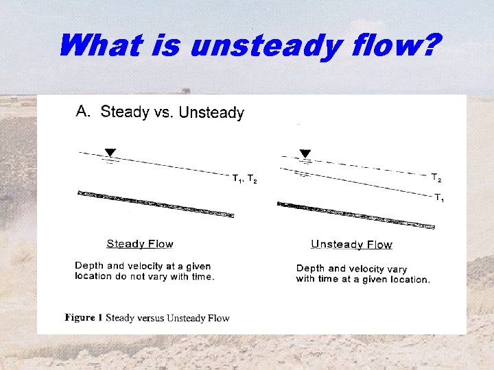
What is unsteady flow?

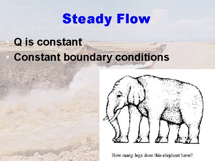
Steady Flow • Q is constant • Constant boundary conditions 4

Unsteady Flow • Q can vary • Constant boundary can vary 5 NRCS watershed program?

HEC-RAS Steady vs. Unsteady • Difference in handling boundary friction and other losses • Difference in numerical solution algorithm • Difference in handling non-flow areas • Difference in flow and boundary condition data requirements • Difference in calibration strategy • Difference in application strategy Keep in mind that finely tuned steady flow data sets may not be optimal for unsteady flow modeling of the same physical setting. 6

Why use HEC-RAS Unsteady Flow? 03 -Nov-20 HEC-RAS Version 3. 1 7

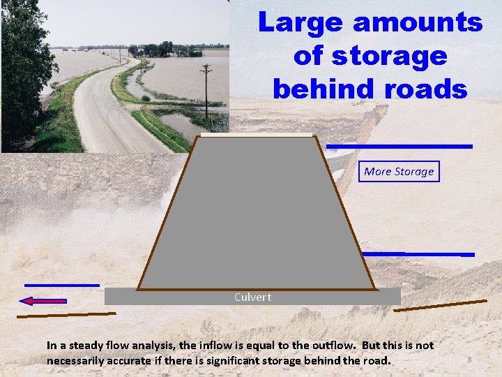
Large amounts of storage behind roads More Storage Culvert In a steady flow analysis, the inflow is equal to the outflow. But this is not necessarily accurate if there is significant storage behind the road. 8

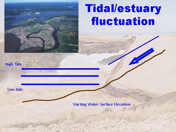
Tidal/estuary fluctuation High Tide Low tide Starting Water Surface Elevation 9

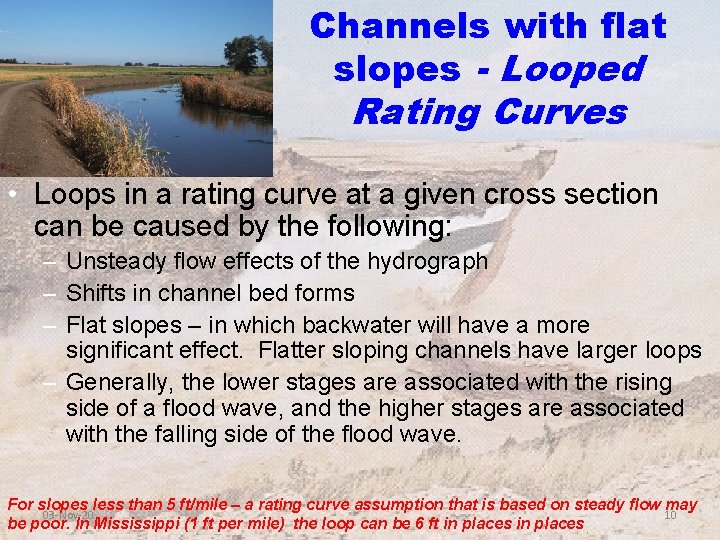
Channels with flat slopes - Looped Rating Curves • Loops in a rating curve at a given cross section can be caused by the following: – Unsteady flow effects of the hydrograph – Shifts in channel bed forms – Flat slopes – in which backwater will have a more significant effect. Flatter sloping channels have larger loops – Generally, the lower stages are associated with the rising side of a flood wave, and the higher stages are associated with the falling side of the flood wave. For slopes less than 5 ft/mile – a rating curve assumption that is based on steady flow may 03 -Nov-20 10 be poor. In Mississippi (1 ft per mile) the loop can be 6 ft in places

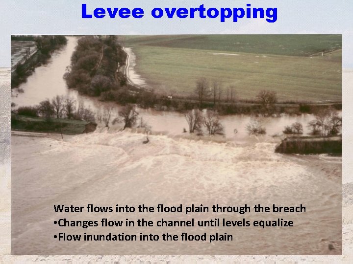
Levee overtopping Water flows into the flood plain through the breach • Changes flow in the channel until levels equalize • Flow inundation into the flood plain 03 -Nov-20 HEC-RAS Version 3. 1 11

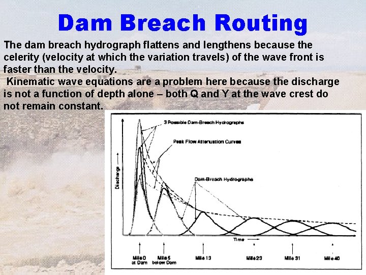
Dam Breach Routing The dam breach hydrograph flattens and lengthens because the celerity (velocity at which the variation travels) of the wave front is faster than the velocity. Kinematic wave equations are a problem here because the discharge is not a function of depth alone – both Q and Y at the wave crest do not remain constant. 12

So why not use unsteady flow modeling for all applications? A: It is hard – debug, very theoretical, bombs, unstable, etc. 03 -Nov-20 HEC-RAS Version 3. 1 13

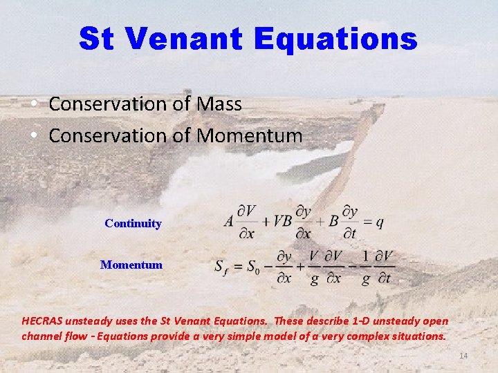
St Venant Equations • Conservation of Mass • Conservation of Momentum Continuity Momentum HECRAS unsteady uses the St Venant Equations. These describe 1 -D unsteady open channel flow - Equations provide a very simple model of a very complex situations. 14

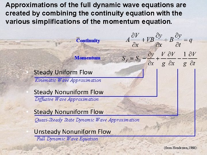
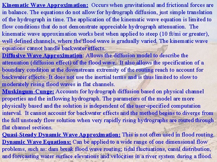
Approximations of the full dynamic wave equations are created by combining the continuity equation with the various simplifications of the momentum equation. Continuity Momentum • Steady Uniform Flow Kinematic Wave Approximation • Steady Nonuniform Flow Diffusive Wave Approximation • Steady Nonuniform Flow Quasi-Steady State Dynamic Wave Approximation • Unsteady Nonuniform Flow Full Dynamic Wave Equation 15 (from Henderson, 1966):

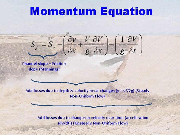
Momentum Equation Channel slope = Friction slope (Mannings) Add losses due to depth & velocity head changes (y + v 2/2 g) (Steady Non-Uniform Flow) Add losses due to changes in velocity over time (acceleration (dv/dt)) (Unsteady Non-Uniform Flow) 16

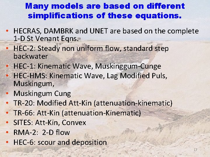
Many models are based on different simplifications of these equations. • HECRAS, DAMBRK and UNET are based on the complete 1 -D St Venant Eqns. • HEC-2: Steady non uniform flow, standard step backwater • HEC-1: Kinematic Wave, Muskinggum-Cunge • HEC-HMS: Kinematic Wave, Lag Modified Puls, Muskingum, • Muskingum Cung • TR-20: Modified Att-Kin (attenuation-kinematic) • TR-66: Att-Kin (attenuation-Kinematic) • SITES: Att-Kin, Convex • RMA-2: 2 -D flow • HEC-6: scour and deposition 17

Kinematic Wave Approximation: Occurs when gravitational and frictional forces are in balance. The equations do not allow for hydrograph diffusion, just simple translation of the hydrograph in time. The application of the kinematic wave equation is limited to flow conditions that do not demonstrate appreciable hydrograph attenuation. The kinematic wave approximation works best when applied to steep (10 ft/mi or greater), well defined channels, where the flood wave is gradually varied. The kinematic wave equations cannot handle backwater effects. Diffusive Wave Approximation: Allows the diffusion model to describe the attenuation (diffusion effect) of the flood wave. It also allows the specification of a boundary condition at the downstream extremity of the routing reach to account for backwater effects. It does not use the inertial terms and is thus limited to slow to moderately rising flood waves in flat channels. Muskingum-Cunge: Accounts for hydrograph diffusion based on physical channel properties and the inflowing hydrograph. The parameters of the model are more physically based and the solution is independent of the user-specified computation interval. It cannot account for backwater effects and the method begins to diverge from the full unsteady flow solution when very rapidly rising hydrographs are routed through flat channel sections. Quasi-Steady Dynamic Wave Approximation: This is not often used in flood routing. Dynamic Wave Equations: Can be applied to a wide range of one dimensional flow problems, such as: dam break flood wave routing; tidal fluctuations, canal distribution, 03 -Nov-20 HEC-RAS Version 3. 1 18 and forecasting water surface elevations and velocities in a river system during a flood.

HEC-RAS Unsteady Flow Computations • HEC-RAS uses a 4 point implicit finite difference scheme using the Newton Raphson iterative technique. • The unsteady flow equation solver was adapted from the UNET model. • The hydraulic calculations for bridges, culverts, and other hydraulic structures that were developed for the steady flow model have been incorporated into the unsteady flow module. • The unsteady flow module has the capability to model storage areas as well as hydraulic connections between storage areas. 19

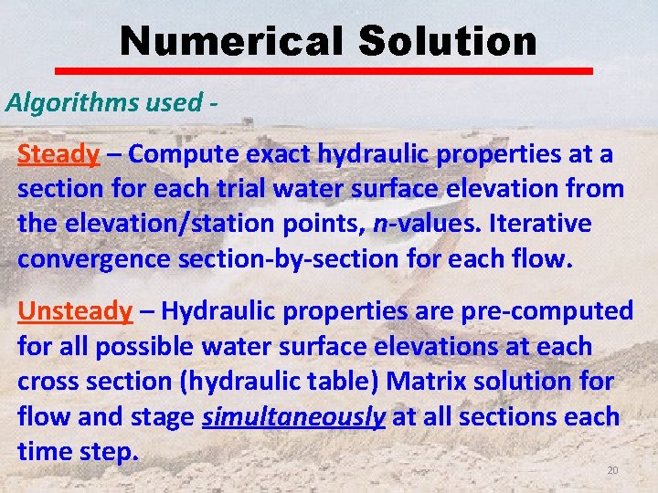
Numerical Solution Algorithms used Steady – Compute exact hydraulic properties at a section for each trial water surface elevation from the elevation/station points, n-values. Iterative convergence section-by-section for each flow. Unsteady – Hydraulic properties are pre-computed for all possible water surface elevations at each cross section (hydraulic table) Matrix solution for flow and stage simultaneously at all sections each time step. 20

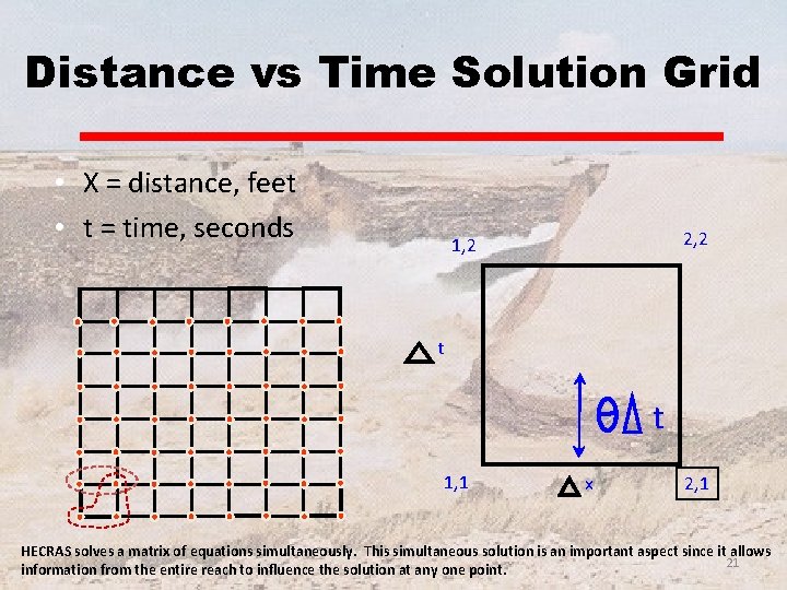
Distance vs Time Solution Grid • X = distance, feet • t = time, seconds 2, 2 1, 2 t t 1, 1 x 2, 1 HECRAS solves a matrix of equations simultaneously. This simultaneous solution is an important aspect since it allows 21 information from the entire reach to influence the solution at any one point.

Bottom Line • Equations used in unsteady modeling are time dependent • A matrix of equations for continuity and momentum are solved simultaneously 22

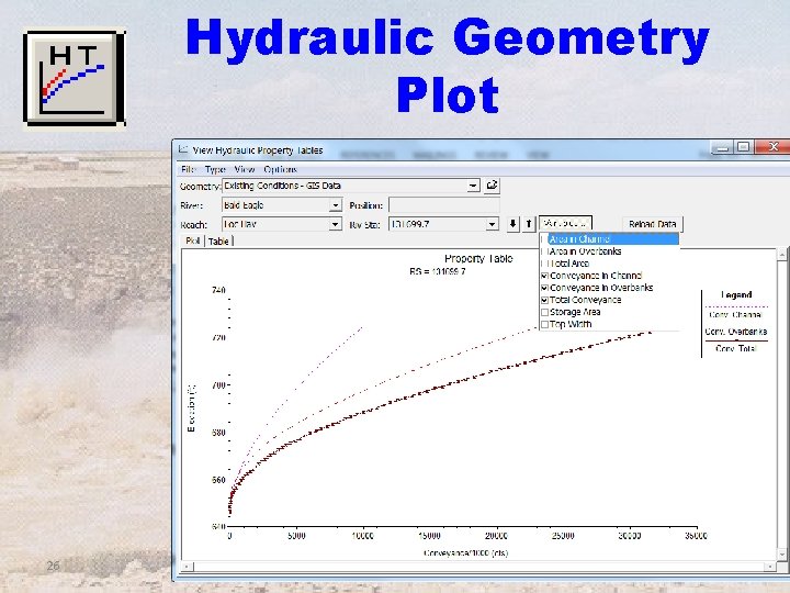
Geometry Preprocessor • For unsteady flow, geometry is preprocessed into tables and rating curves – Cross sections are processed into tables of area, conveyance, and storage – Bridges and culverts are processed into a family of rating curves for each structure – Weirs and gated structures are calculated on the fly during unsteady flow calculations – Pre-processor results can be viewed in graphs and tables 23

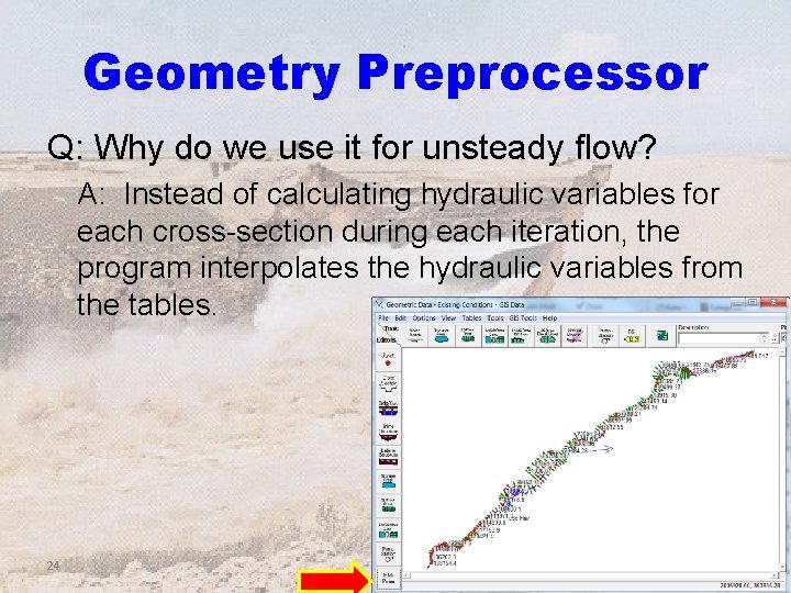
Geometry Preprocessor Q: Why do we use it for unsteady flow? A: Instead of calculating hydraulic variables for each cross-section during each iteration, the program interpolates the hydraulic variables from the tables. 24

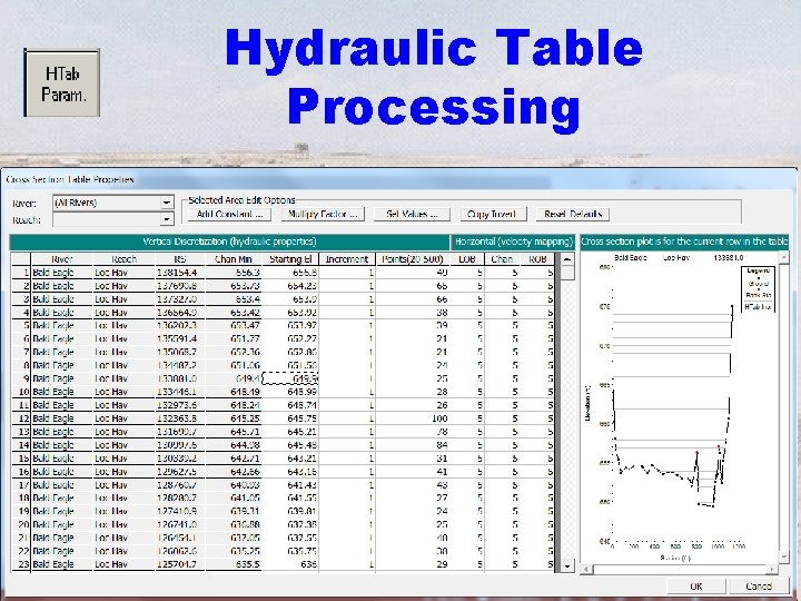
Hydraulic Table Processing 25

Hydraulic Geometry Plot 26

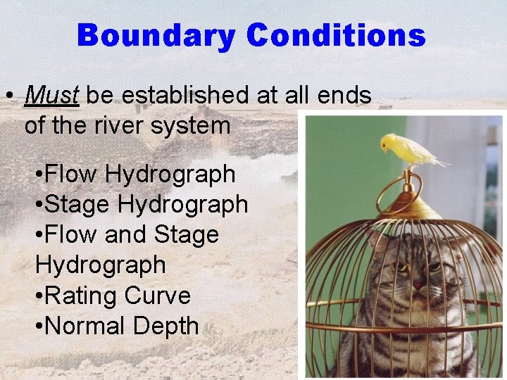
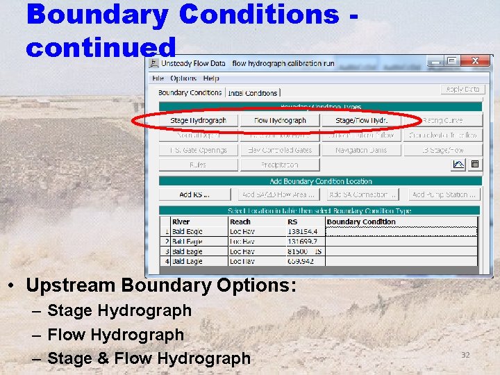
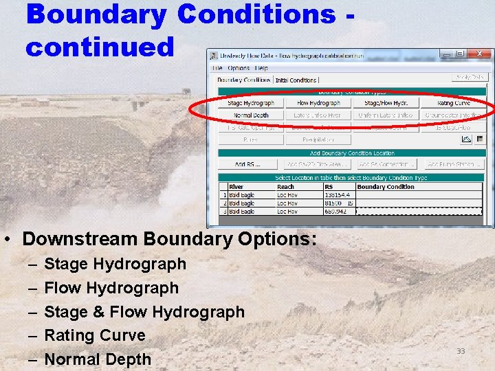
Boundary Conditions • Must be established at all ends of the river system • Flow Hydrograph • Stage Hydrograph • Flow and Stage Hydrograph • Rating Curve • Normal Depth 27

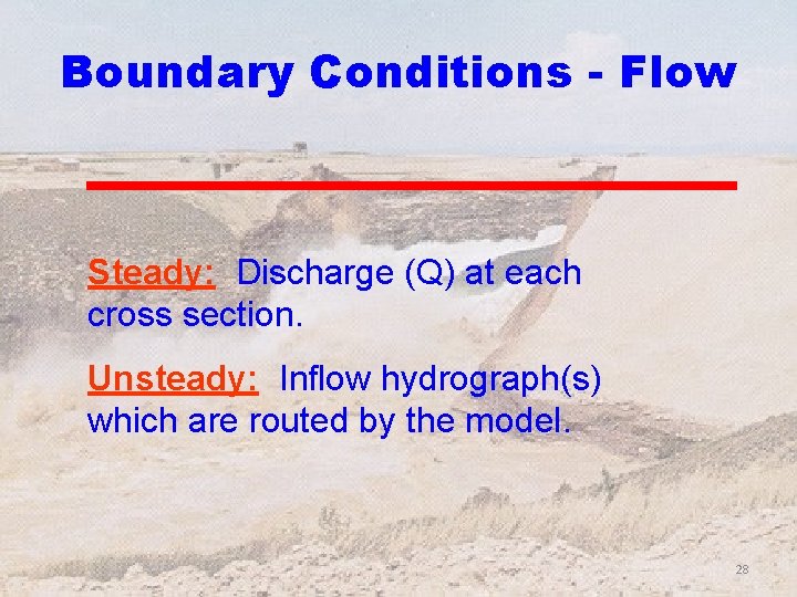
Boundary Conditions - Flow Steady: Discharge (Q) at each cross section. Unsteady: Inflow hydrograph(s) which are routed by the model. 28

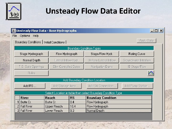
Unsteady Flow Data Editor 29

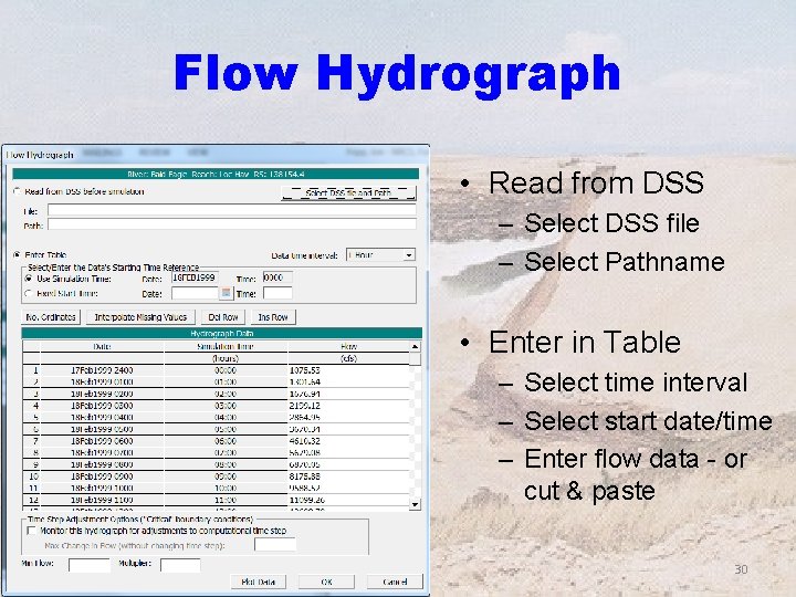
Flow Hydrograph • Read from DSS – Select DSS file – Select Pathname • Enter in Table – Select time interval – Select start date/time – Enter flow data - or cut & paste 30

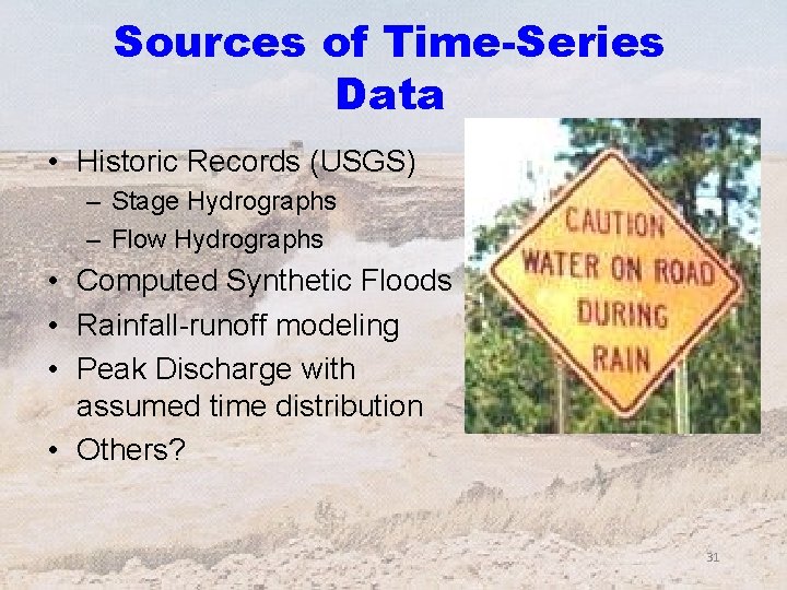
Sources of Time-Series Data • Historic Records (USGS) – Stage Hydrographs – Flow Hydrographs • Computed Synthetic Floods • Rainfall-runoff modeling • Peak Discharge with assumed time distribution • Others? 31

Boundary Conditions continued • Upstream Boundary Options: – Stage Hydrograph – Flow Hydrograph – Stage & Flow Hydrograph 32

Boundary Conditions continued • Downstream Boundary Options: – – – Stage Hydrograph Flow Hydrograph Stage & Flow Hydrograph Rating Curve Normal Depth 33

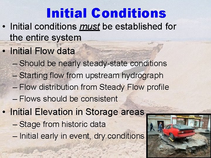
Initial Conditions • Initial conditions must be established for the entire system • Initial Flow data – Should be nearly steady-state conditions – Starting flow from upstream hydrograph – Flow distribution from Steady Flow profile – Flows should be consistent • Initial Elevation in Storage areas – Stage from historic data – Initial early in event, dry conditions 34

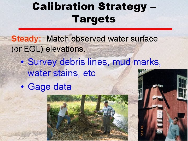
Calibration Strategy – Targets Steady: Match observed water surface (or EGL) elevations. • Survey debris lines, mud marks, water stains, etc • Gage data

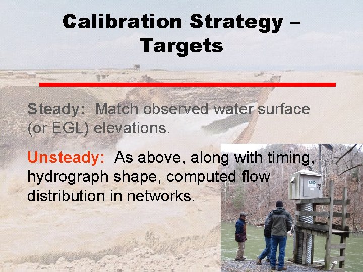
Calibration Strategy – Targets Steady: Match observed water surface (or EGL) elevations. Unsteady: As above, along with timing, hydrograph shape, computed flow distribution in networks.

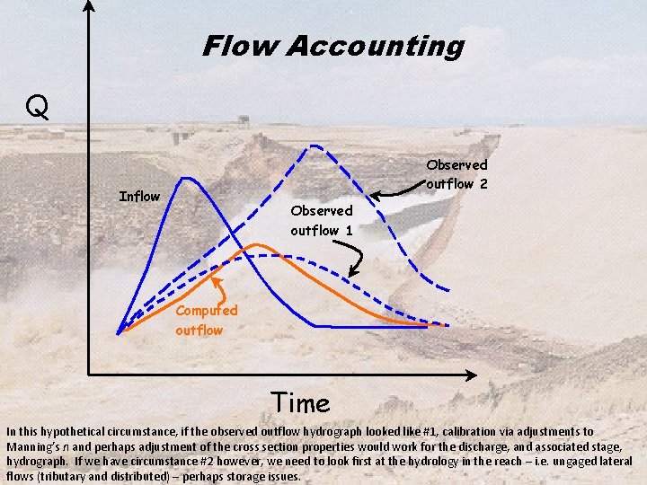
Flow Accounting Q Observed outflow 2 Inflow Observed outflow 1 Computed outflow Time In this hypothetical circumstance, if the observed outflow hydrograph looked like #1, calibration via adjustments to Manning’s n and perhaps adjustment of the cross section properties would work for the discharge, and associated stage, hydrograph. If we have circumstance #2 however, we need to look first at the hydrology in the reach – i. e. ungaged lateral flows (tributary and distributed) – perhaps storage issues.

Procedure 1. Develop a Steady Flow Model 2. Calibrate it to steady flow 3. Develop the unsteady flow model 4. Calibrate it to unsteady flow 38

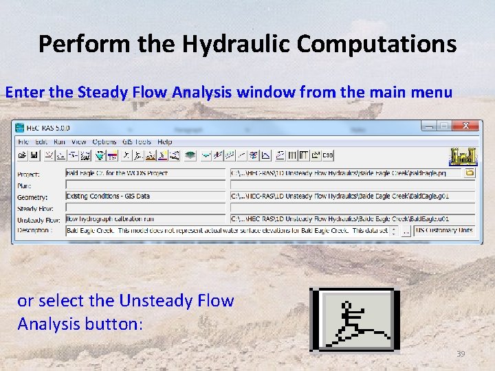
Perform the Hydraulic Computations Enter the Steady Flow Analysis window from the main menu or select the Unsteady Flow Analysis button: 39

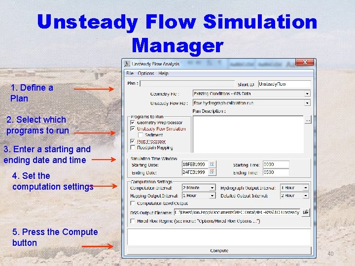
Unsteady Flow Simulation Manager 1. Define a Plan 2. Select which programs to run 3. Enter a starting and ending date and time 4. Set the computation settings 5. Press the Compute button 40

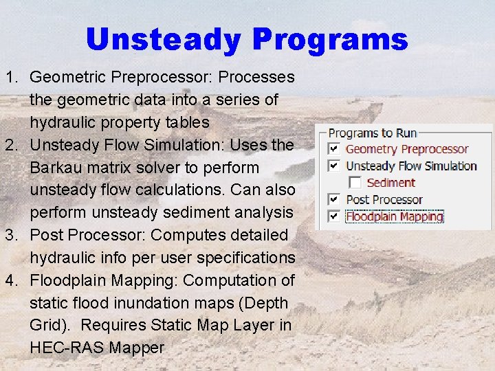
Unsteady Programs 1. Geometric Preprocessor: Processes the geometric data into a series of hydraulic property tables 2. Unsteady Flow Simulation: Uses the Barkau matrix solver to perform unsteady flow calculations. Can also perform unsteady sediment analysis 3. Post Processor: Computes detailed hydraulic info per user specifications 4. Floodplain Mapping: Computation of static flood inundation maps (Depth Grid). Requires Static Map Layer in HEC-RAS Mapper

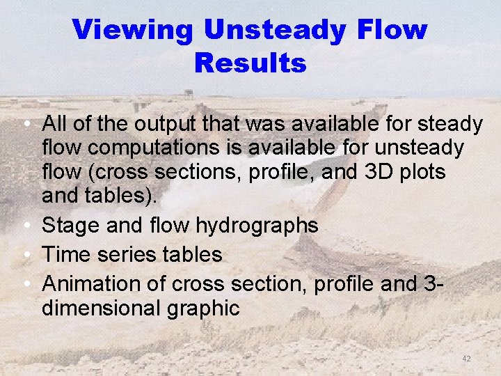
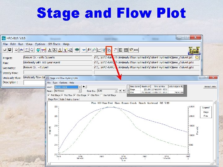
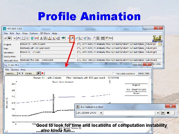
Viewing Unsteady Flow Results • All of the output that was available for steady flow computations is available for unsteady flow (cross sections, profile, and 3 D plots and tables). • Stage and flow hydrographs • Time series tables • Animation of cross section, profile and 3 dimensional graphic 42

Stage and Flow Plot Stage 43

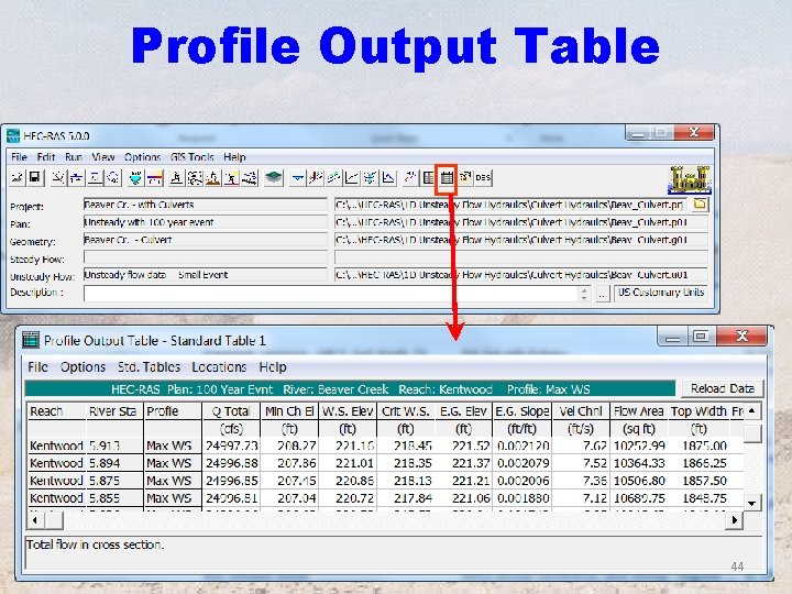
Profile Output Table 44

Profile Animation Good to look for time and locations of computation instability 45 …also kinda fun…

Model Accuracy • Accuracy can be defined as the degree of closeness of the numerical solution to the true solution. • Accuracy depends upon the following: – Assumptions and limitations of the model (i. e. one dimensional model, subcritical flow only for unsteady flow) – Accuracy of the geometric Data (cross sections, Manning’s n values, bridges, culverts, etc…) – Accuracy of the flow data and boundary conditions – Numerical Accuracy of the solution scheme 46

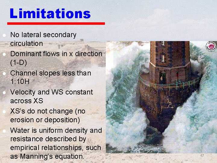
Limitations l l l No lateral secondary circulation Dominant flows in x direction (1 -D) Channel slopes less than 1: 10 H Velocity and WS constant across XS XS’s do not change (no erosion or deposition) Water is uniform density and resistance described by empirical relationships, such as Manning’s equation. 47

Unsteady modeling can be difficult… Be careful 48

Unsteady Flow Documentation • Technical/theoretical - Chapters 2 and 5 from EM 1110 -2 -1416 • http: //www. hnd. usace. army. mil - click on TECHINFO, then Engineering Publications, then Engineering Manuals, scroll for manual • HEC-RAS User’s Manual - Chapter 8 (data input and window operations) • HEC-RAS Application Guide - Chapter 17 (example application) 49

The End You may need some help 50