HECRAS Basic Steady 1 D Flow HECRAS Data

HEC-RAS Basic Steady 1 D Flow ~ HECRAS Data Input / Output Jon Fripp NDCSMC 2016

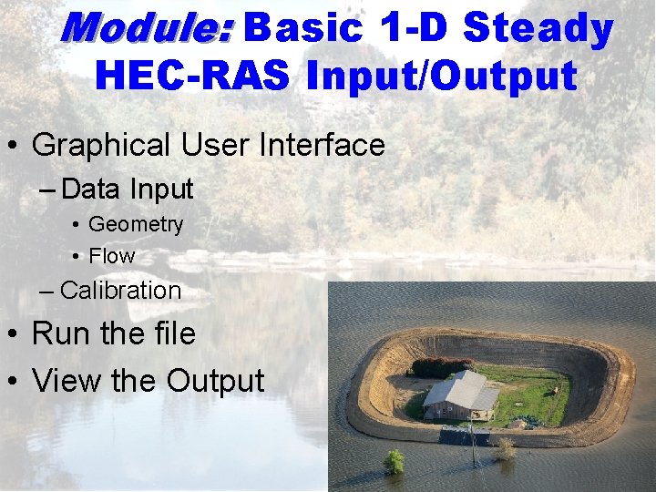
Module: Basic 1 -D Steady HEC-RAS Input/Output • Graphical User Interface – Data Input • Geometry • Flow – Calibration • Run the file • View the Output

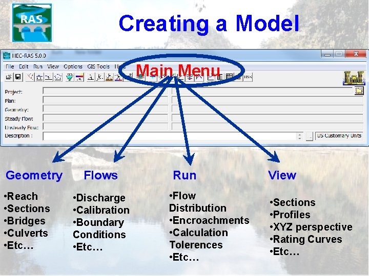
Creating a Model Main Menu The HECRAS Model Geometry • Reach • Sections • Bridges • Culverts • Etc… Flows • Discharge • Calibration • Boundary Conditions • Etc… Run • Flow Distribution • Encroachments • Calculation Tolerences • Etc… View • Sections • Profiles • XYZ perspective • Rating Curves • Etc…

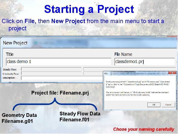
Starting a Project Click on File, then New Project from the main menu to start a project Project file: Filename. prj Geometry Data Filename. g 01 Steady Flow Data Filename. f 01 Chose your naming carefully

Geometry

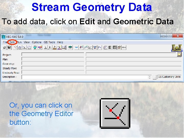
Stream Geometry Data To add data, click on Edit and Geometric Data Or, you can click on the Geometry Editor button:

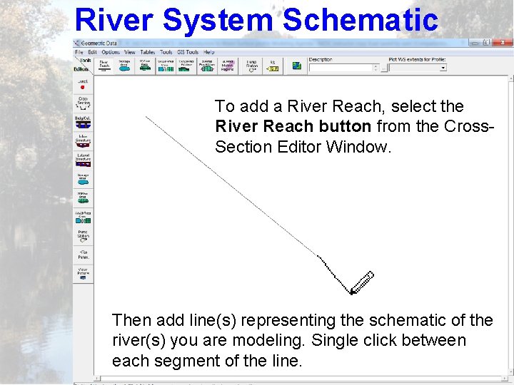
River System Schematic To add a River Reach, select the River Reach button from the Cross. Section Editor Window. Then add line(s) representing the schematic of the river(s) you are modeling. Single click between each segment of the line.

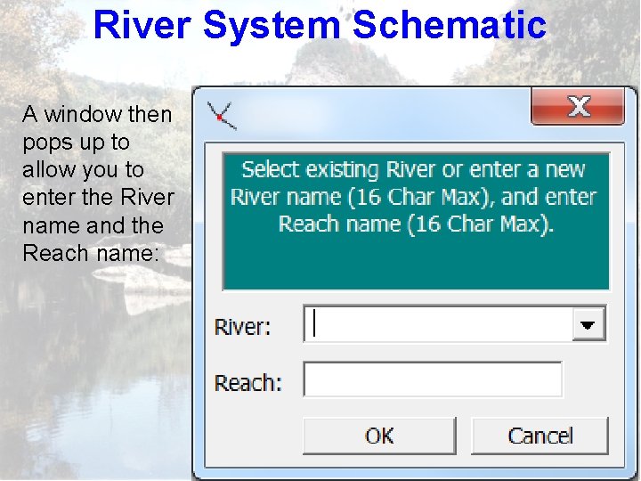
River System Schematic A window then pops up to allow you to enter the River name and the Reach name:

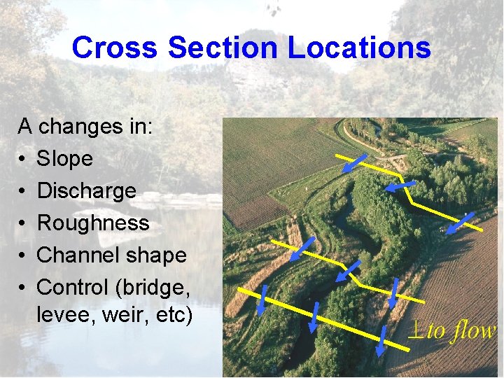
Cross Section Locations A changes in: • Slope • Discharge • Roughness • Channel shape • Control (bridge, levee, weir, etc)

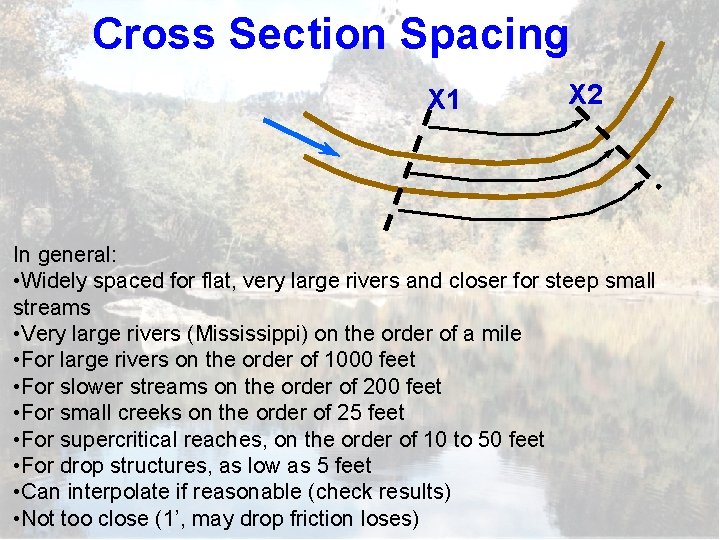
Cross Section Spacing X 1 X 2 In general: • Widely spaced for flat, very large rivers and closer for steep small streams • Very large rivers (Mississippi) on the order of a mile • For large rivers on the order of 1000 feet • For slower streams on the order of 200 feet • For small creeks on the order of 25 feet • For supercritical reaches, on the order of 10 to 50 feet • For drop structures, as low as 5 feet • Can interpolate if reasonable (check results) • Not too close (1’, may drop friction loses)

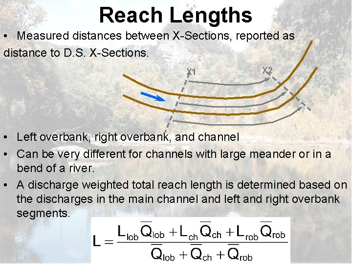
Reach Lengths • Measured distances between X-Sections, reported as distance to D. S. X-Sections. X 1 X 2 • Left overbank, right overbank, and channel • Can be very different for channels with large meander or in a bend of a river. • A discharge weighted total reach length is determined based on the discharges in the main channel and left and right overbank segments.

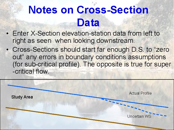
Notes on Cross-Section Data • Enter X-Section elevation-station data from left to right as seen when looking downstream. • Cross-Sections should start far enough D. S. to “zero out” any errors in boundary conditions assumptions (for sub-critical profile). The opposite is true for super -critical flow. Study Area Actual Profile Uncertain WS

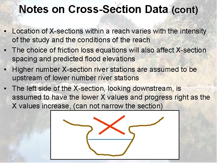
Notes on Cross-Section Data (cont) • Location of X-sections within a reach varies with the intensity of the study and the conditions of the reach • The choice of friction loss equations will also affect X-section spacing and predicted flood elevations • Higher number X-section river stations are assumed to be upstream of lower number river stations • The left side of the X-section, looking downstream, is assumed to have the lower X values and progress right as the X values increase, (can not narrow the section)

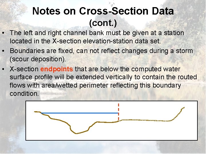
Notes on Cross-Section Data (cont. ) • The left and right channel bank must be given at a station located in the X-section elevation-station data set. • Boundaries are fixed, can not reflect changes during a storm (scour deposition). • X-section endpoints that are below the computed water surface profile will be extended vertically to contain the routed flows with area/wetted perimeter reflecting this boundary condition.

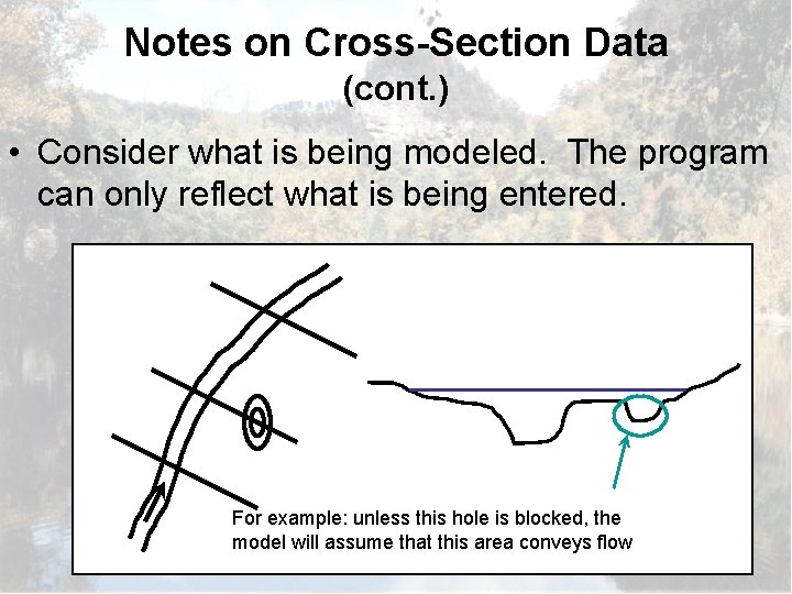
Notes on Cross-Section Data (cont. ) • Consider what is being modeled. The program can only reflect what is being entered. For example: unless this hole is blocked, the model will assume that this area conveys flow

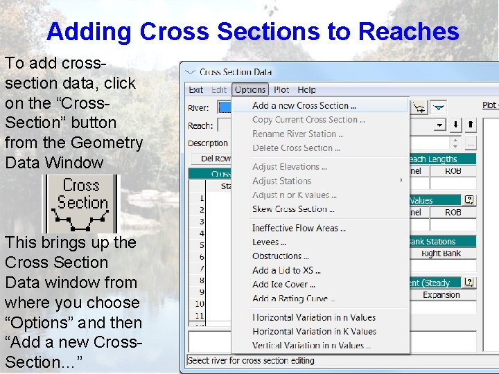
Adding Cross Sections to Reaches To add crosssection data, click on the “Cross. Section” button from the Geometry Data Window This brings up the Cross Section Data window from where you choose “Options” and then “Add a new Cross. Section…”

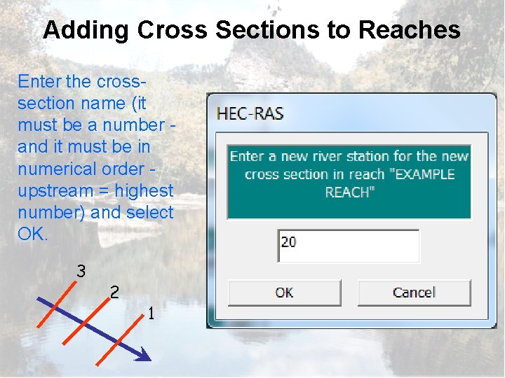
Adding Cross Sections to Reaches Enter the crosssection name (it must be a number and it must be in numerical order upstream = highest number) and select OK. 3 2 1

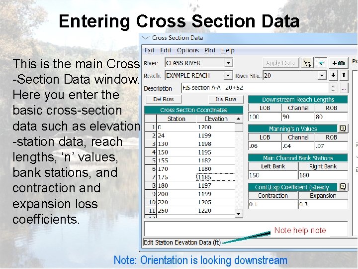
Entering Cross Section Data This is the main Cross -Section Data window. Here you enter the basic cross-section data such as elevation -station data, reach lengths, ‘n’ values, bank stations, and contraction and expansion loss coefficients. Note help note Note: Orientation is looking downstream

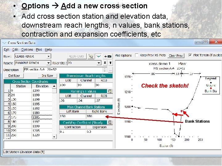
• Options Add a new cross section • Add cross section station and elevation data, downstream reach lengths, n values, bank stations, contraction and expansion coefficients, etc. Check the sketch! Bank Stations

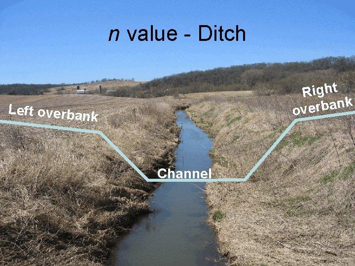
n value - Ditch Right k n a b r e ov Left overban k Channel

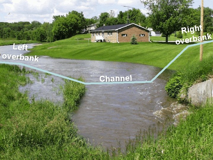
Urban stream n value Left overbank Channel Right k n a b r e ov

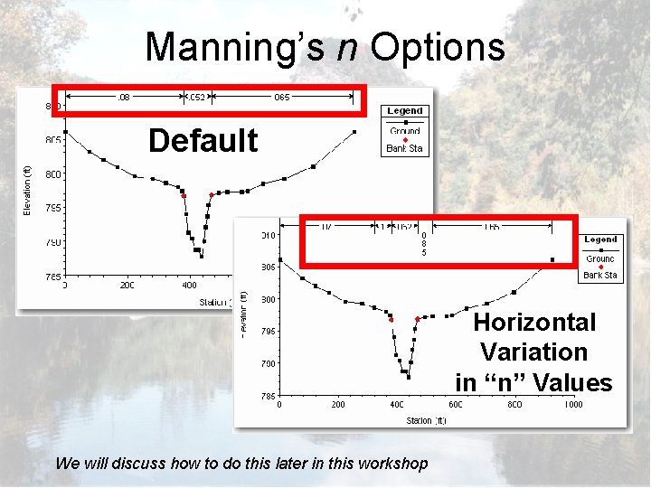
Manning’s n Options Default Horizontal Variation in “n” Values We will discuss how to do this later in this workshop

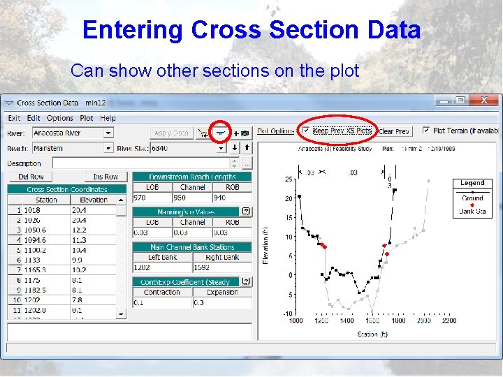
Entering Cross Section Data Can show other sections on the plot

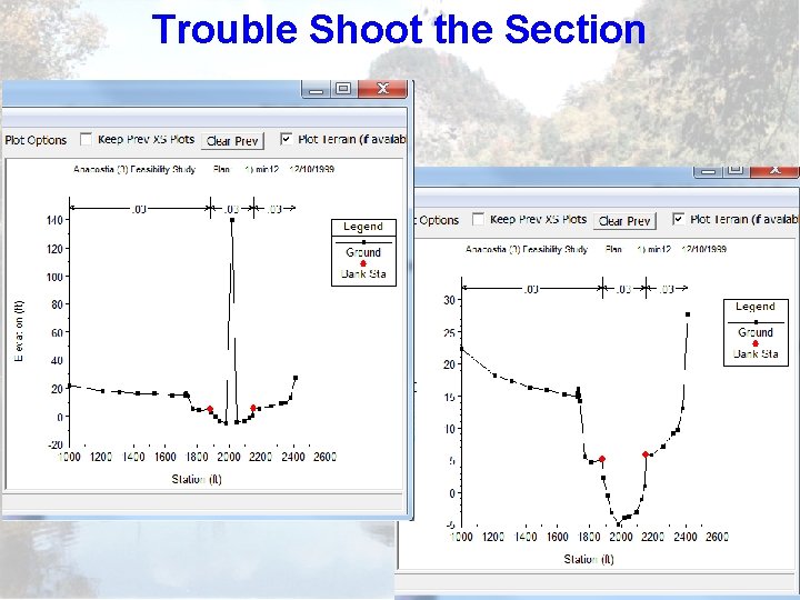
Trouble Shoot the Section

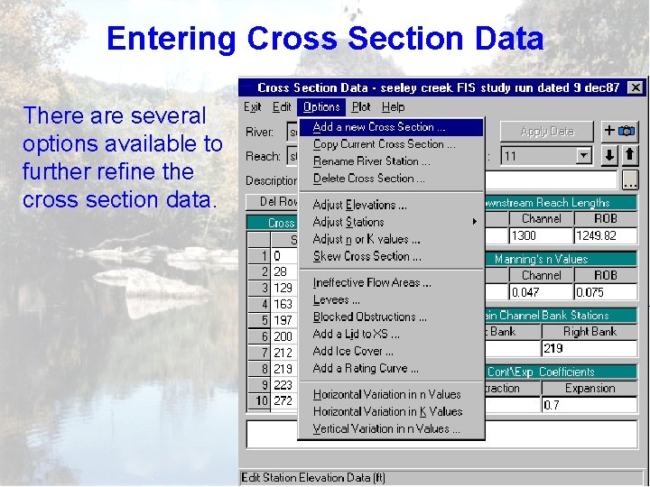
Entering Cross Section Data There are several options available to further refine the cross section data.

Ineffective Flow Areas • Ineffective flow areas are used to model portions of the cross-section in which water will pond, but the velocity of that water in the downstream direction is equal to zero. • This water is included in the storage and wetted cross section parameters, but not in the active flow area. • No additional wetted parameter is added to the active flow area (unlike encroachments). • Once ineffective flow area is overtopped, then that specific area is no longer considered ineffective. • Commonly used near road crossings. Think of them as dead storage zones

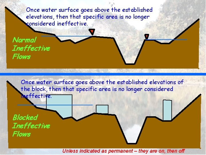
Once water surface goes above the established elevations, then that specific area is no longer considered ineffective. Normal Ineffective Flows Once water surface goes above the established elevations of the block, then that specific area is no longer considered ineffective. Blocked Ineffective Flows Unless indicated as permanent – they are on, then off

Blocked Obstructions • Used to define areas that will be permanently blocked out. • Decreases flow area and increases wetted perimeter when the water comes in contact with it. • Two types of blocked obstructions are available Normal and Multiple. They are very similar to the Ineffective Flow areas, except that the blocked areas are never available as water flow areas. • Water can get to the off-sides of these obstructions. Think of them as part of the section

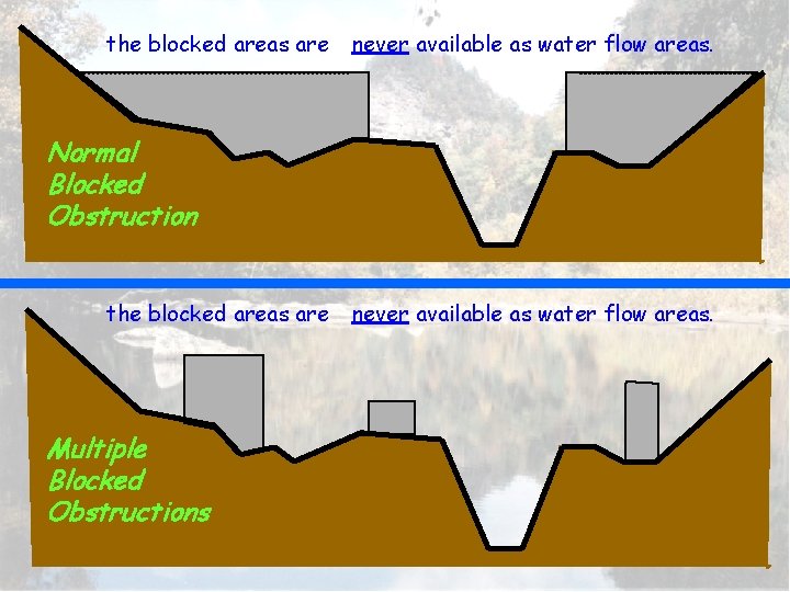
the blocked areas are never available as water flow areas. Normal Blocked Obstruction the blocked areas are Multiple Blocked Obstructions never available as water flow areas.

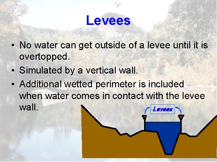
Levees • No water can get outside of a levee until it is overtopped. • Simulated by a vertical wall. • Additional wetted perimeter is included when water comes in contact with the levee wall. Levees

Levees vs. Ineffective Flow Areas Ineffective flow areas is used where water is present to the left/right of the ineffective station but the velocity is zero. Volume included in storage and wetted perimeter calculations but not in conveyance. (think: ponded area) • A levee acts as a vertical wall. No water occupied the space to the left/right of the levee unless the levee elevation is exceeded. The distance that the levee is in contact with the water is included in the wetted perimeter calculations. (think: wall)

Flow Data

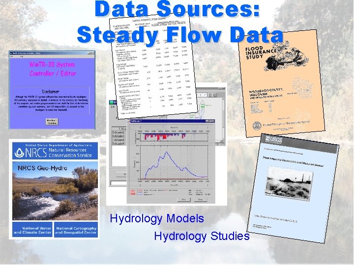
Data Sources: Steady Flow Data Hydrology Models Hydrology Studies

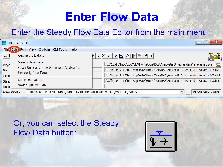
Enter Flow Data Enter the Steady Flow Data Editor from the main menu Or, you can select the Steady Flow Data button:

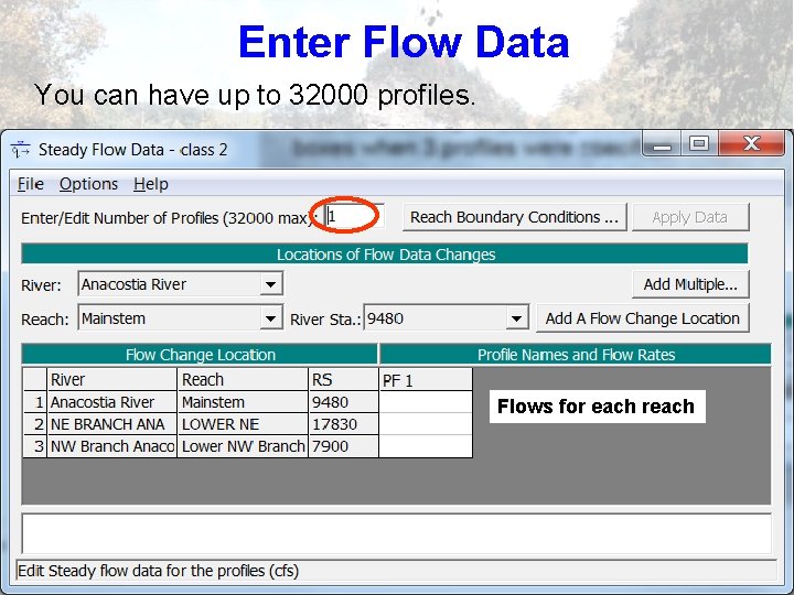
Enter Flow Data You can have up to 32000 profiles. Flows for each reach

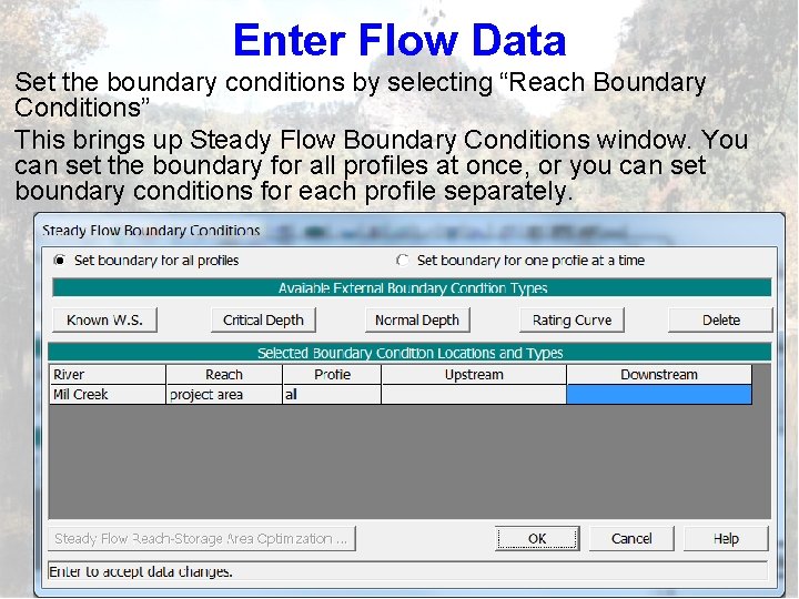
Enter Flow Data Set the boundary conditions by selecting “Reach Boundary Conditions” This brings up Steady Flow Boundary Conditions window. You can set the boundary for all profiles at once, or you can set boundary conditions for each profile separately.

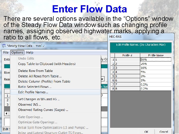
Enter Flow Data There are several options available in the “Options” window of the Steady Flow Data window such as changing profile names, assigning observed highwater marks, applying a ratio to all flows, etc.

Calibration: A Definition • Calibration is the adjustment of a model's parameters, such as roughness, and hydraulic structure coefficients, so that it reproduces observed prototype data to an acceptable accuracy.

Calibration Strategy – Targets Steady: Match observed water surface (or EGL) elevations.

Sources of observed data • Survey debris lines, mud marks, water stains, etc • Gage data

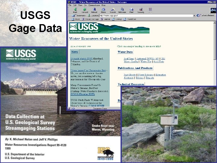
USGS Gage Data Surface Water

Stage Records • Most accurate hydrologic input. Generally known within +/- 1. 0 foot. • Possible Errors: – Float gage gets stuck at a specific stage. – Recording systematically accumulates error with time. – Gage reader misses several days and guesses at stage recordings. – Error in the datum of the gage. – Changes in stream/river management – Changes in stream/river morphology

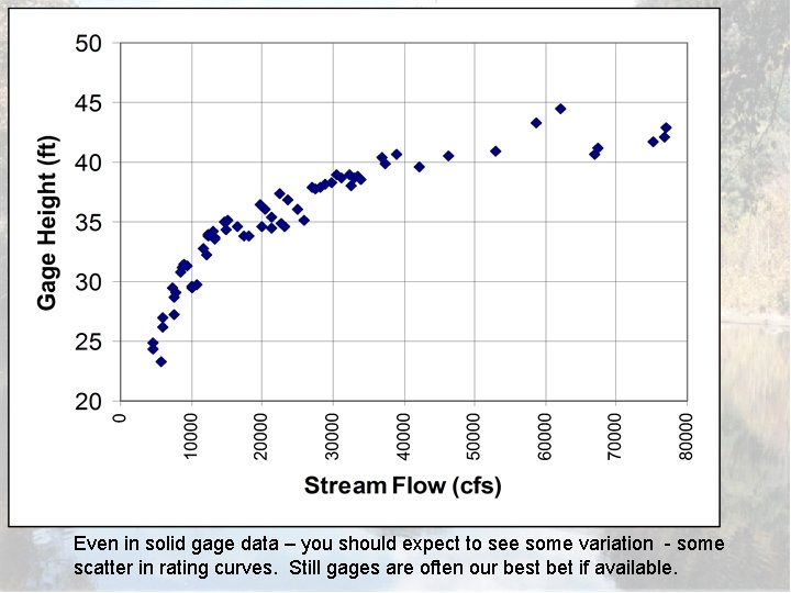
Even in solid gage data – you should expect to see some variation - some scatter in rating curves. Still gages are often our best bet if available.

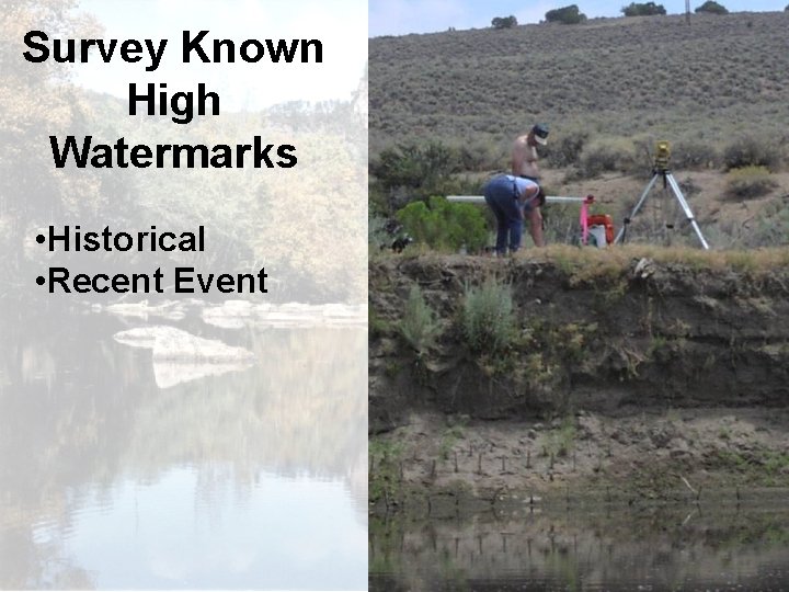
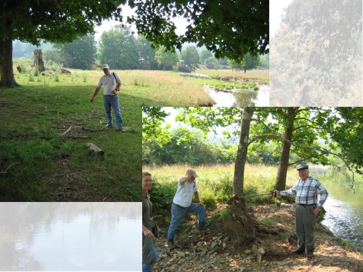
Survey Known High Watermarks • Historical • Recent Event

Cautions with the use of High Water Marks • Wind and wave actions can cause the debris lines to be higher than the actual water surface. • Capillary action causes stains on buildings to migrate upward. • High water marks in the overbank area are often higher than in the channel. Overbank water is moving slower and may be closer to energy gradline. • High water marks on bridge piers are often equal to the energy gradeline, not the average water surface.

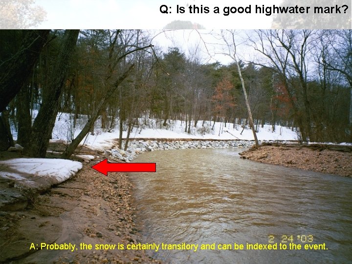
Q: Is this a good highwater mark? A: Probably, the snow is certainly transitory and can be indexed to the event.

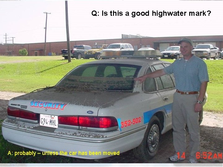
Q: Is this a good highwater mark? A: probably – unless the car has been moved

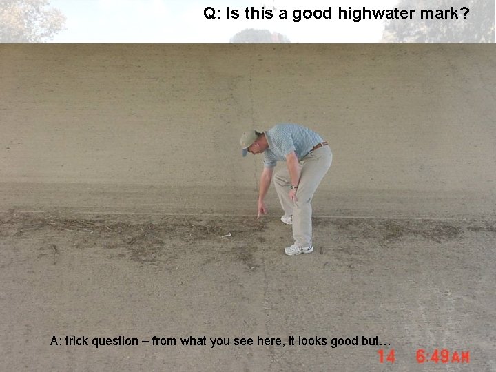
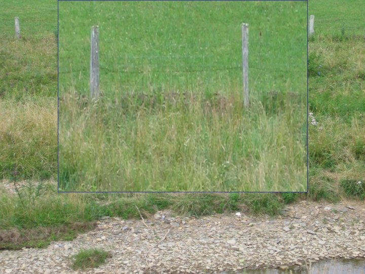
Q: Is this a good highwater mark? A: trick question – from what you see here, it looks good but…

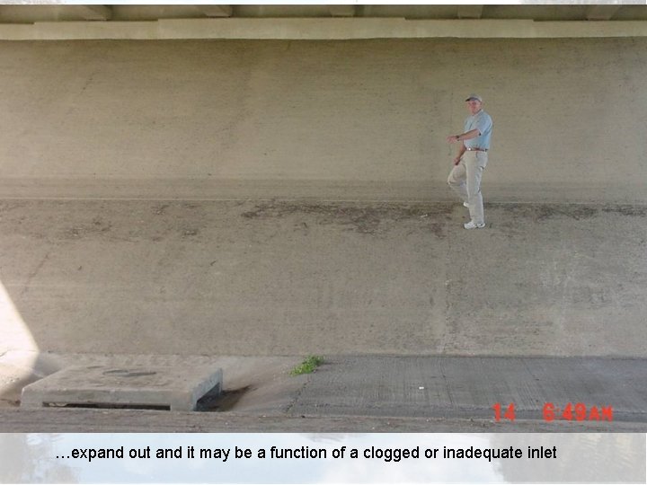
…expand out and it may be a function of a clogged or inadequate inlet

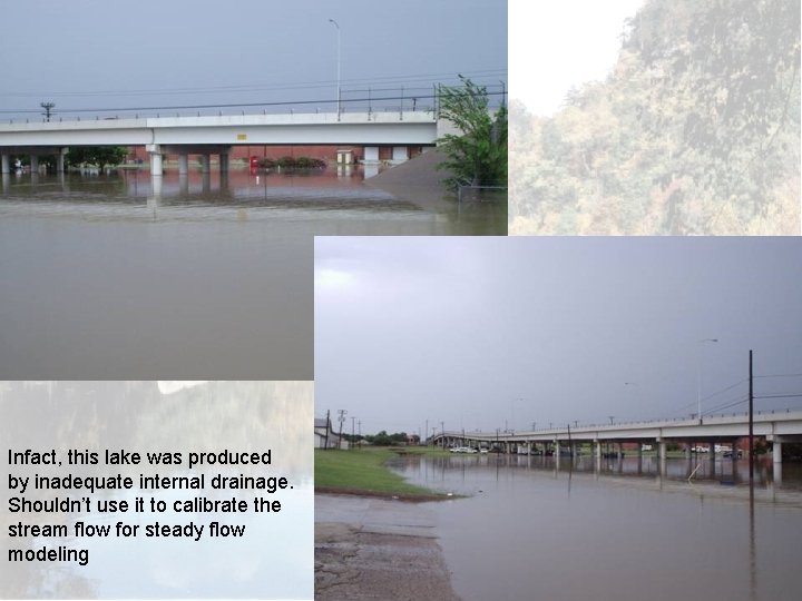
Infact, this lake was produced by inadequate internal drainage. Shouldn’t use it to calibrate the stream flow for steady flow modeling

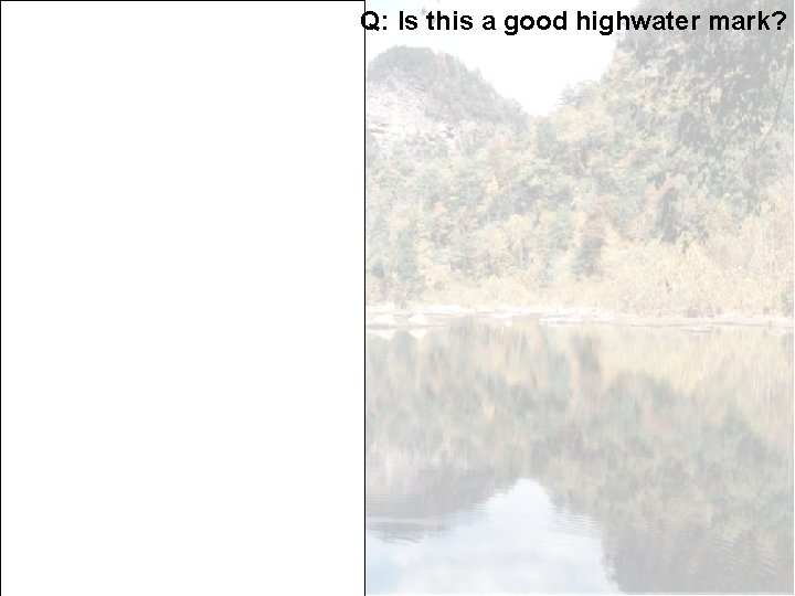
Q: Is this a good highwater mark? Honduras - photo from John Tiedeman

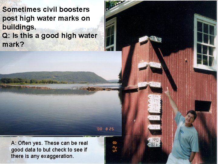
Sometimes civil boosters post high water marks on buildings. Q: Is this a good high water mark? A: Often yes. These can be real good data to but check to see if there is any exaggeration.

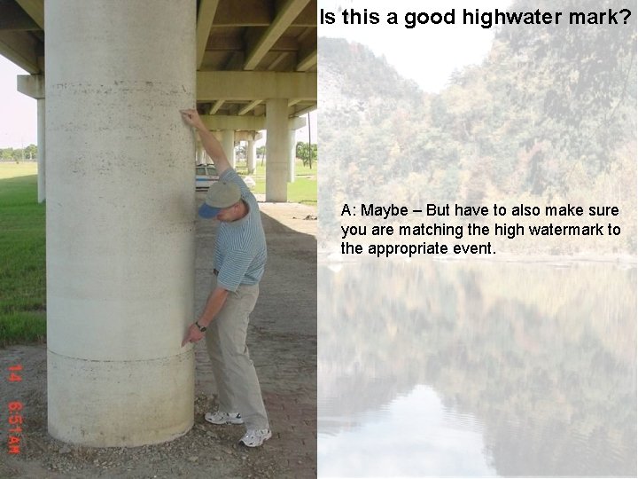
Q: Is this a good highwater mark? A: Maybe – But have to also make sure you are matching the high watermark to the appropriate event.

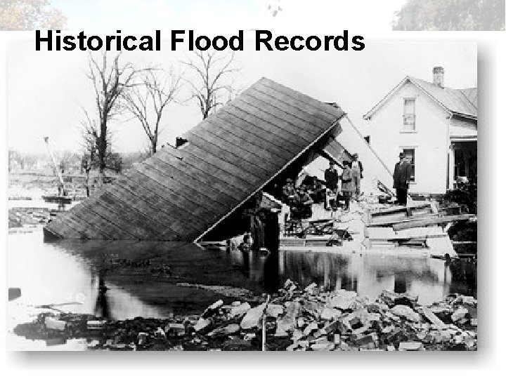
Historical Flood Records

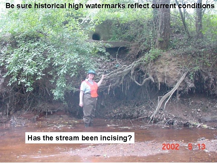
Be sure historical high watermarks reflect current conditions Has the stream been incising?

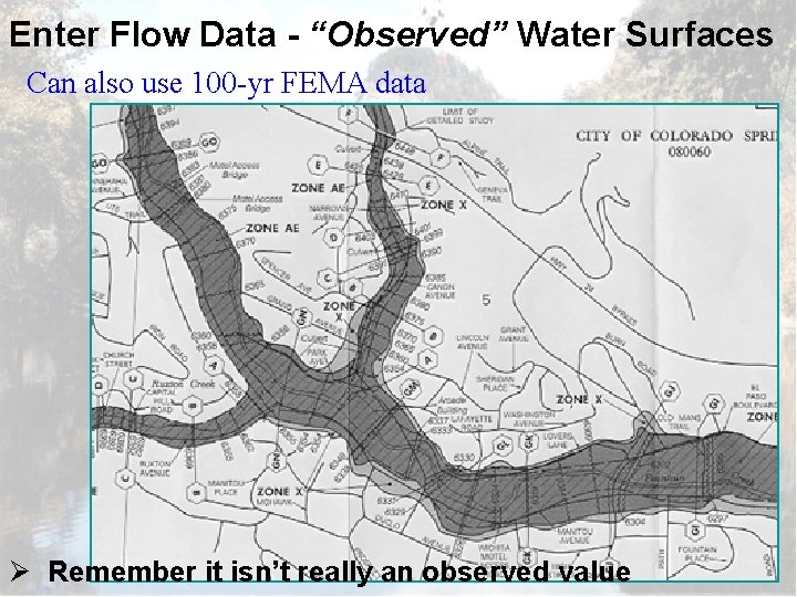
Enter Flow Data - “Observed” Water Surfaces Can also use 100 -yr FEMA data Ø Remember it isn’t really an observed value

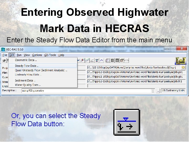
Entering Observed Highwater Mark Data in HECRAS Enter the Steady Flow Data Editor from the main menu Or, you can select the Steady Flow Data button:

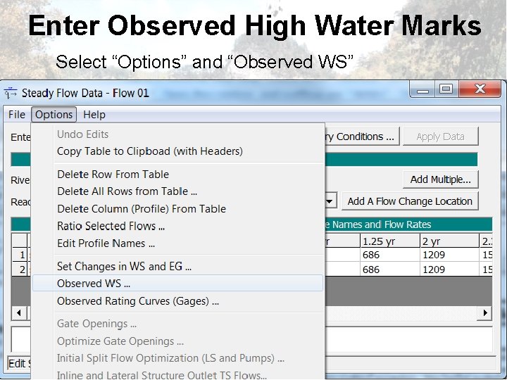
Enter Observed High Water Marks Select “Options” and “Observed WS”

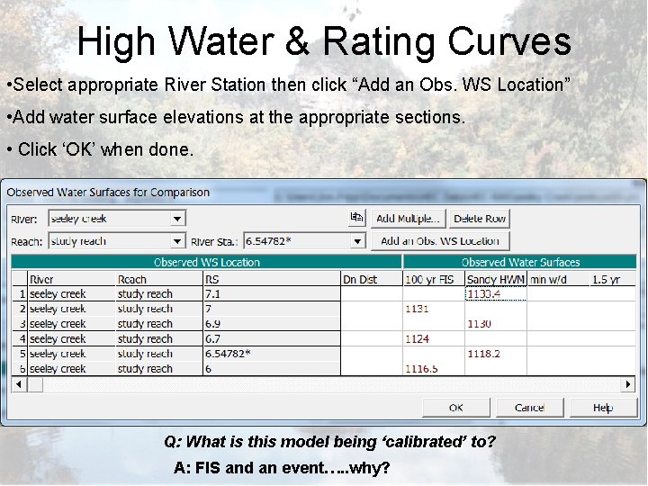
High Water & Rating Curves • Select appropriate River Station then click “Add an Obs. WS Location” • Add water surface elevations at the appropriate sections. • Click ‘OK’ when done. Q: What is this model being ‘calibrated’ to? A: FIS and an event…. . why?

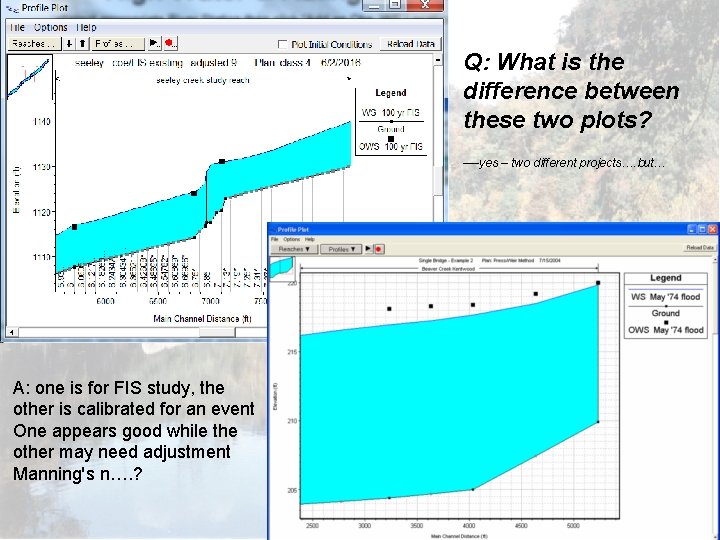
Q: What is the difference between these two plots? ----yes – two different projects…. but… A: one is for FIS study, the other is calibrated for an event One appears good while the other may need adjustment Manning's n…. ?

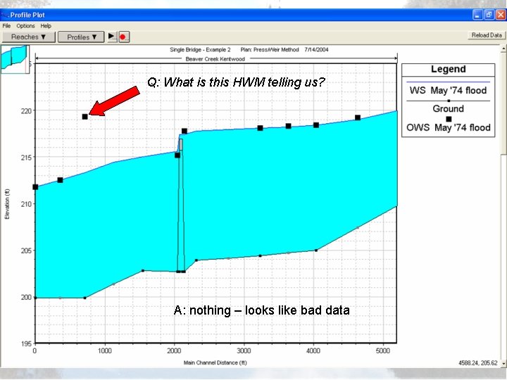
Q: What is this HWM telling us? A: nothing – looks like bad data

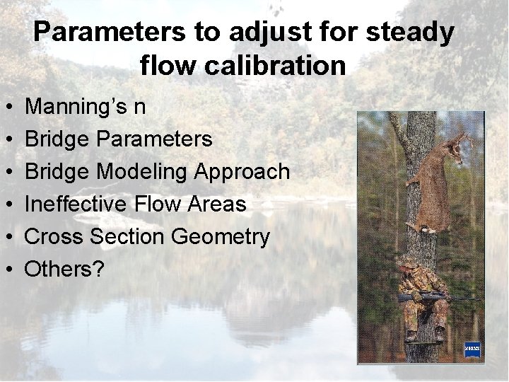
Parameters to adjust for steady flow calibration • • • Manning’s n Bridge Parameters Bridge Modeling Approach Ineffective Flow Areas Cross Section Geometry Others?

Greatest problem is inconsistency: A HECRAS model will reproduce one event but not another.

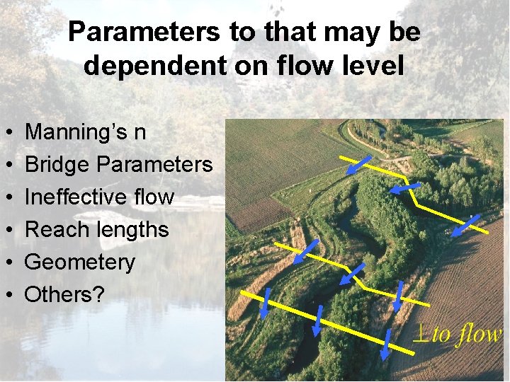
Parameters to that may be dependent on flow level • • • Manning’s n Bridge Parameters Ineffective flow Reach lengths Geometery Others?

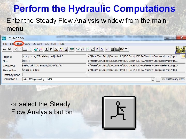
Perform the Hydraulic Computations Enter the Steady Flow Analysis window from the main menu or select the Steady Flow Analysis button:

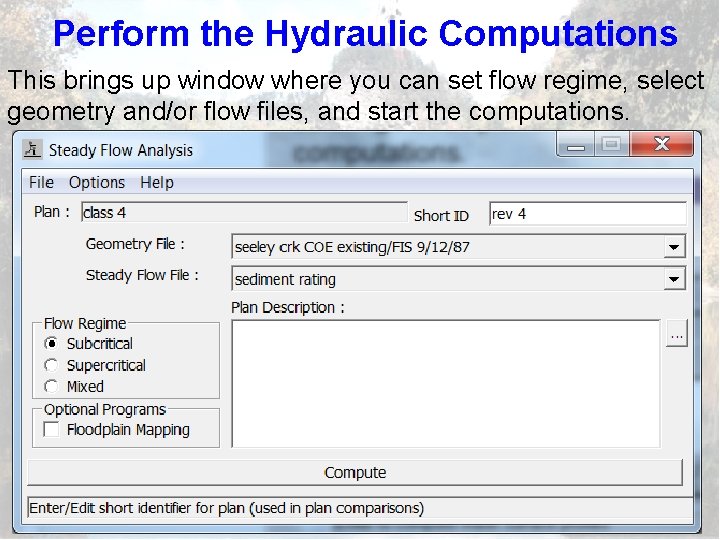
Perform the Hydraulic Computations This brings up window where you can set flow regime, select geometry and/or flow files, and start the computations.

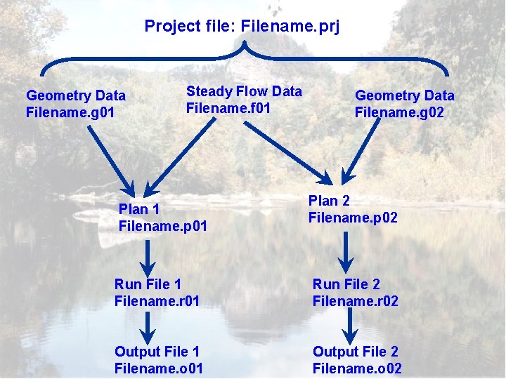
Project file: Filename. prj Geometry Data Filename. g 01 Steady Flow Data Filename. f 01 Plan 1 Filename. p 01 Geometry Data Filename. g 02 Plan 2 Filename. p 02 Run File 1 Filename. r 01 Run File 2 Filename. r 02 Output File 1 Filename. o 01 Output File 2 Filename. o 02

Viewing the Output • • Graphical Tabular Profile Section

View the Output There are several output formats to view within the view menu such as plotted cross-sections, profiles, rating curves and 3 -D views as well as cross-section and profile tabular data.

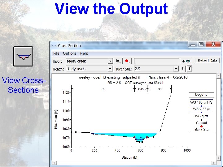
View the Output View Cross. Sections

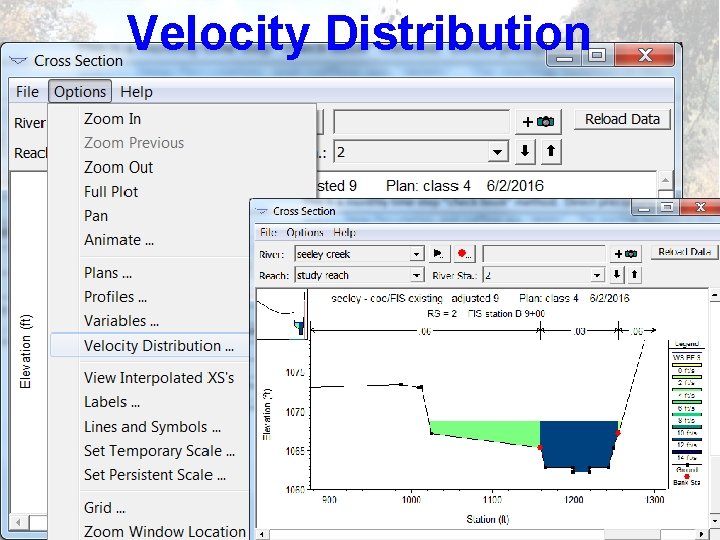
Velocity Distribution

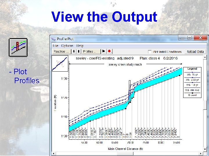
View the Output - Plot Profiles

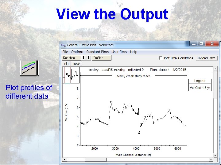
View the Output Plot profiles of different data

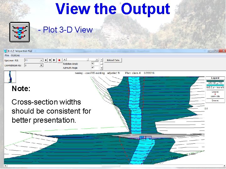
View the Output - Plot 3 -D View Note: Cross-section widths should be consistent for better presentation.

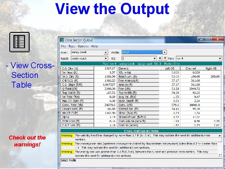
View the Output - View Cross. Section Table Check out the warnings!

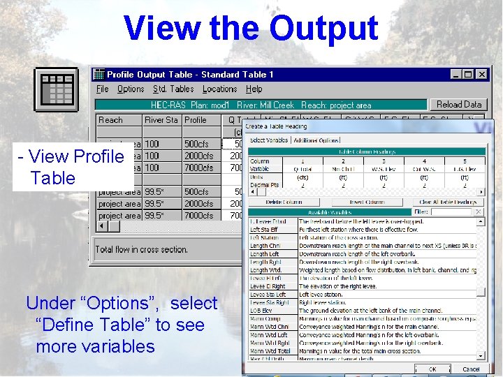
View the Output - View Profile Table Under “Options”, select “Define Table” to see more variables

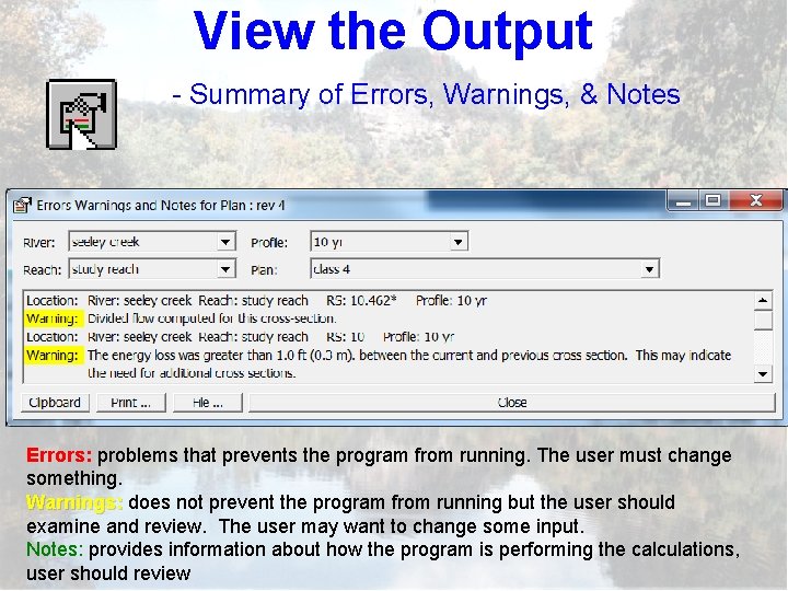
View the Output - Summary of Errors, Warnings, & Notes Errors: problems that prevents the program from running. The user must change something. Warnings: does not prevent the program from running but the user should examine and review. The user may want to change some input. Notes: provides information about how the program is performing the calculations, user should review

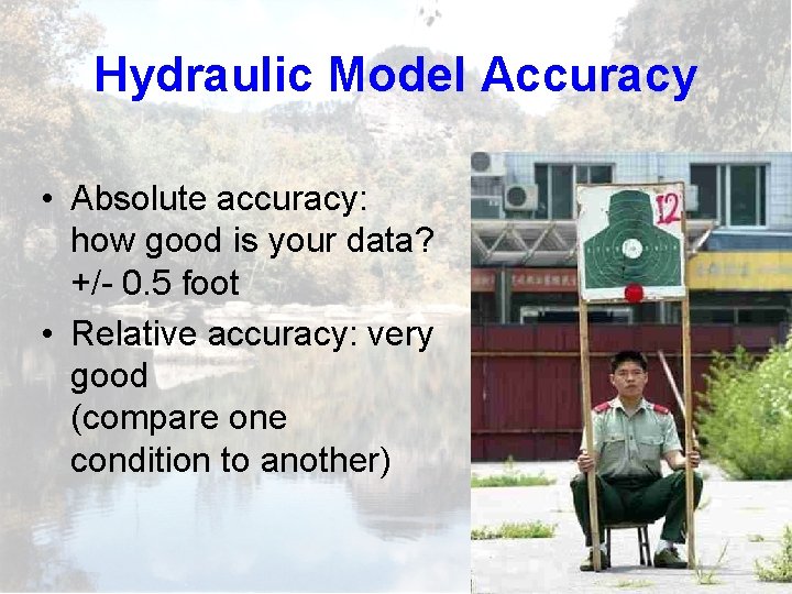
Hydraulic Model Accuracy • Absolute accuracy: how good is your data? +/- 0. 5 foot • Relative accuracy: very good (compare one condition to another)

The End Questions?