Handling Outliers and Missing Data in Statistical Data

Handling Outliers and Missing Data in Statistical Data Models Kaushik Mitra Date: 17/1/2011 ECSU Seminar, ISI

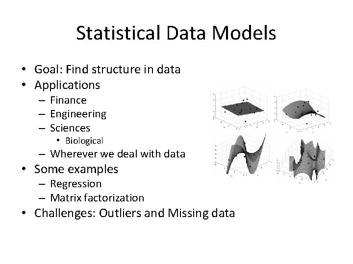
Statistical Data Models • Goal: Find structure in data • Applications – Finance – Engineering – Sciences • Biological – Wherever we deal with data • Some examples – Regression – Matrix factorization • Challenges: Outliers and Missing data

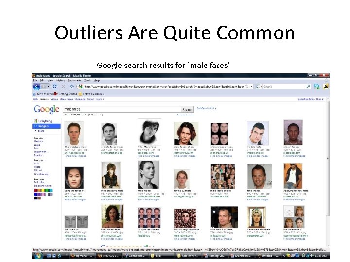
Outliers Are Quite Common Google search results for `male faces’

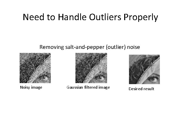
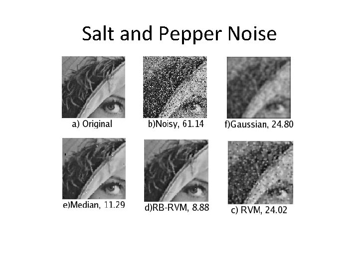
Need to Handle Outliers Properly Removing salt-and-pepper (outlier) noise Noisy image Gaussian filtered image Desired result

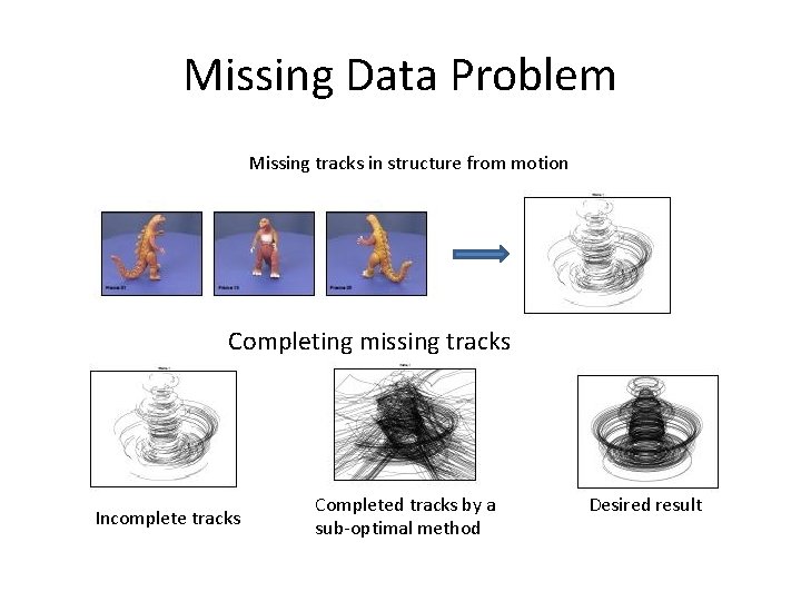
Missing Data Problem Missing tracks in structure from motion Completing missing tracks Incomplete tracks Completed tracks by a sub-optimal method Desired result

Our Focus • Outliers in regression – Linear regression – Kernel regression • Matrix factorization in presence of missing data

Robust Linear Regression for High Dimension Problems

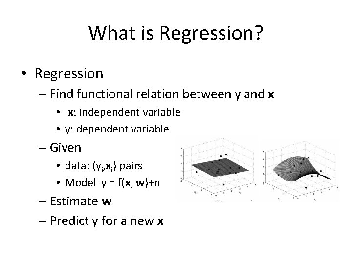
What is Regression? • Regression – Find functional relation between y and x • x: independent variable • y: dependent variable – Given • data: (yi, xi) pairs • Model y = f(x, w)+n – Estimate w – Predict y for a new x

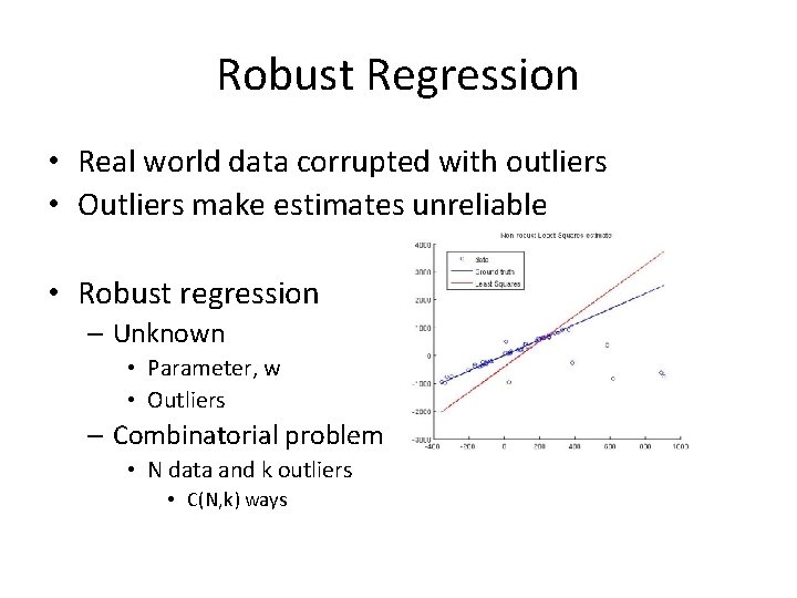
Robust Regression • Real world data corrupted with outliers • Outliers make estimates unreliable • Robust regression – Unknown • Parameter, w • Outliers – Combinatorial problem • N data and k outliers • C(N, k) ways

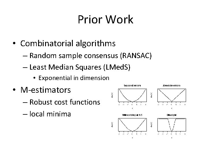
Prior Work • Combinatorial algorithms – Random sample consensus (RANSAC) – Least Median Squares (LMed. S) • Exponential in dimension • M-estimators – Robust cost functions – local minima

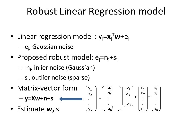
Robust Linear Regression model • Linear regression model : yi=xi. Tw+ei – ei, Gaussian noise • Proposed robust model: ei=ni+si – ni, inlier noise (Gaussian) – si, outlier noise (sparse) • Matrix-vector form – y=Xw+n+s • Estimate w, s y 1 y 2. . y. N = x 1 T x 2 T. . x. N T w 1 w 2 +. w. D n 1 s 1 n 2 s 2. +. . . n. N s. N

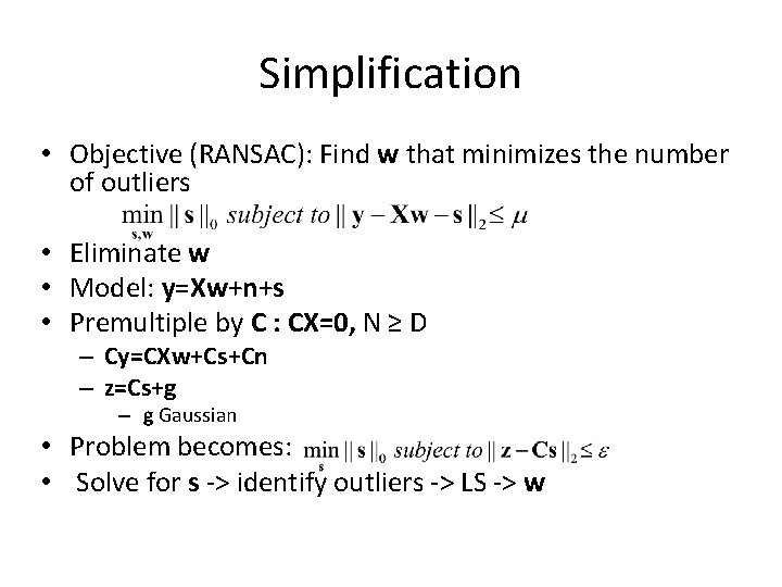
Simplification • Objective (RANSAC): Find w that minimizes the number of outliers • Eliminate w • Model: y=Xw+n+s • Premultiple by C : CX=0, N ≥ D – Cy=CXw+Cs+Cn – z=Cs+g – g Gaussian • Problem becomes: • Solve for s -> identify outliers -> LS -> w

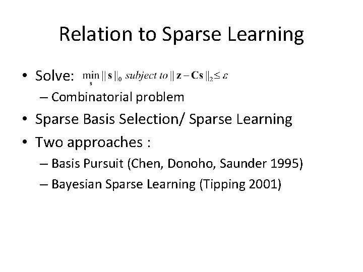
Relation to Sparse Learning • Solve: – Combinatorial problem • Sparse Basis Selection/ Sparse Learning • Two approaches : – Basis Pursuit (Chen, Donoho, Saunder 1995) – Bayesian Sparse Learning (Tipping 2001)

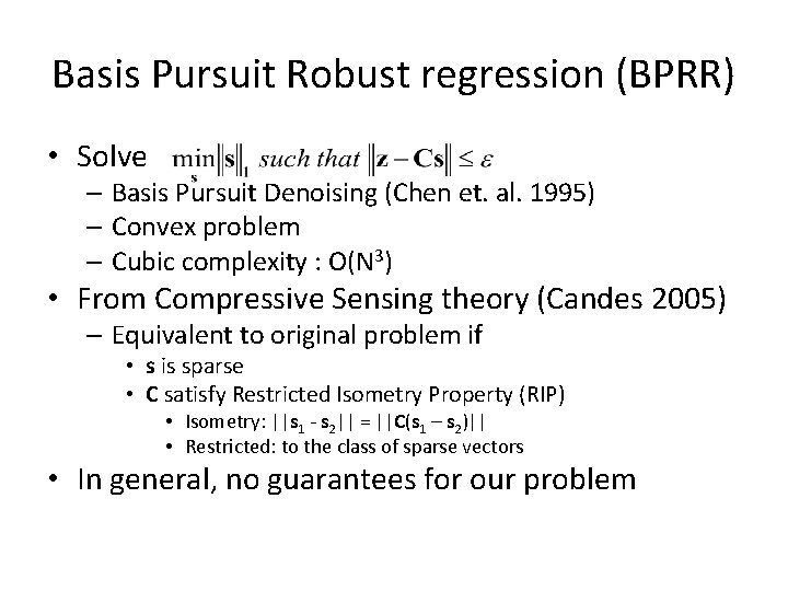
Basis Pursuit Robust regression (BPRR) • Solve – Basis Pursuit Denoising (Chen et. al. 1995) – Convex problem – Cubic complexity : O(N 3) • From Compressive Sensing theory (Candes 2005) – Equivalent to original problem if • s is sparse • C satisfy Restricted Isometry Property (RIP) • Isometry: ||s 1 - s 2|| = ||C(s 1 – s 2)|| • Restricted: to the class of sparse vectors • In general, no guarantees for our problem

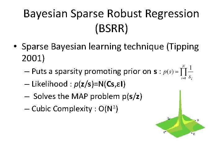
Bayesian Sparse Robust Regression (BSRR) • Sparse Bayesian learning technique (Tipping 2001) – Puts a sparsity promoting prior on s : – Likelihood : p(z/s)=Ν(Cs, εI) – Solves the MAP problem p(s/z) – Cubic Complexity : O(N 3)

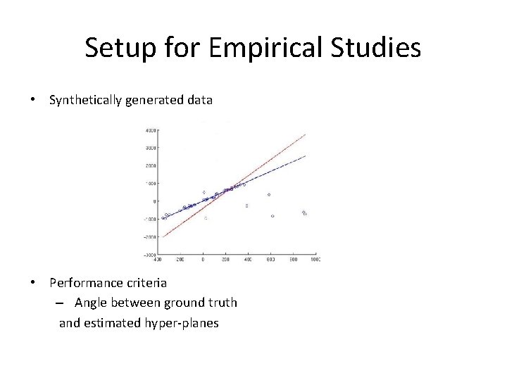
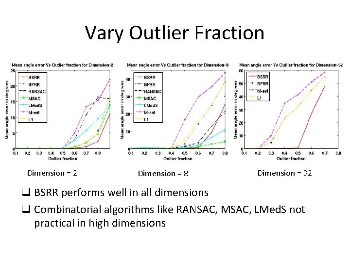
Setup for Empirical Studies • Synthetically generated data • Performance criteria – Angle between ground truth and estimated hyper-planes

Vary Outlier Fraction Dimension = 2 Dimension = 8 Dimension = 32 q BSRR performs well in all dimensions q Combinatorial algorithms like RANSAC, MSAC, LMed. S not practical in high dimensions

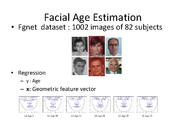
Facial Age Estimation • Fgnet dataset : 1002 images of 82 subjects • Regression – y : Age – x: Geometric feature vector

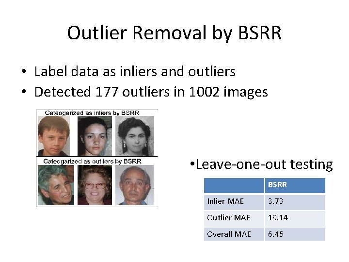
Outlier Removal by BSRR • Label data as inliers and outliers • Detected 177 outliers in 1002 images • Leave-one-out testing BSRR Inlier MAE 3. 73 Outlier MAE 19. 14 Overall MAE 6. 45

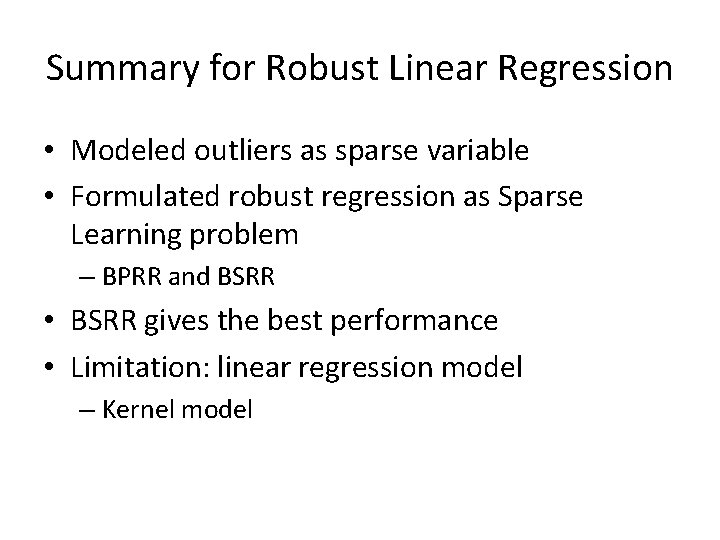
Summary for Robust Linear Regression • Modeled outliers as sparse variable • Formulated robust regression as Sparse Learning problem – BPRR and BSRR • BSRR gives the best performance • Limitation: linear regression model – Kernel model

Robust RVM Using Sparse Outlier Model

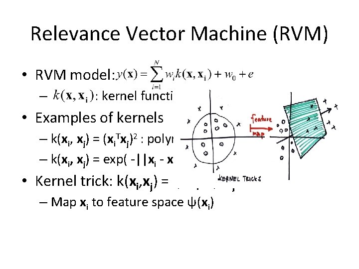
Relevance Vector Machine (RVM) • RVM model: – : kernel function • Examples of kernels – k(xi, xj) = (xi. Txj)2 : polynomial kernel – k(xi, xj) = exp( -||xi - xj||2/2σ2) : Gaussian kernel • Kernel trick: k(xi, xj) = ψ(xi)Tψ(xj) – Map xi to feature space ψ(xi)

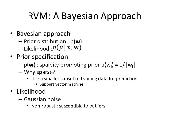
RVM: A Bayesian Approach • Bayesian approach – Prior distribution : p(w) – Likelihood : • Prior specification – p(w) : sparsity promoting prior p(wi) = 1/|wi| – Why sparse? • Use a smaller subset of training data for prediction • Support vector machine • Likelihood – Gaussian noise • Non-robust : susceptible to outliers

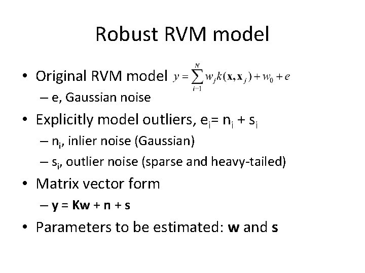
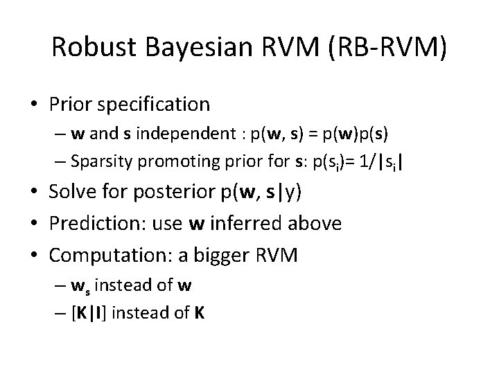
Robust RVM model • Original RVM model – e, Gaussian noise • Explicitly model outliers, ei= ni + si – ni, inlier noise (Gaussian) – si, outlier noise (sparse and heavy-tailed) • Matrix vector form – y = Kw + n + s • Parameters to be estimated: w and s

Robust RVM Algorithms • y = [K|I]ws + n – ws = [w. T s. T]T : sparse vector • Two approaches – Bayesian – Optimization

Robust Bayesian RVM (RB-RVM) • Prior specification – w and s independent : p(w, s) = p(w)p(s) – Sparsity promoting prior for s: p(si)= 1/|si| • Solve for posterior p(w, s|y) • Prediction: use w inferred above • Computation: a bigger RVM – ws instead of w – [K|I] instead of K

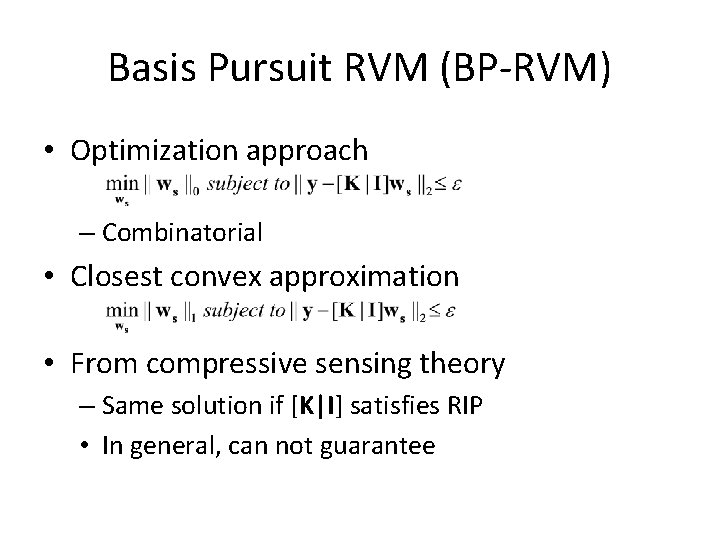
Basis Pursuit RVM (BP-RVM) • Optimization approach – Combinatorial • Closest convex approximation • From compressive sensing theory – Same solution if [K|I] satisfies RIP • In general, can not guarantee

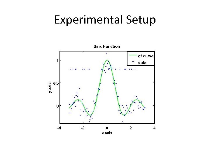
Experimental Setup

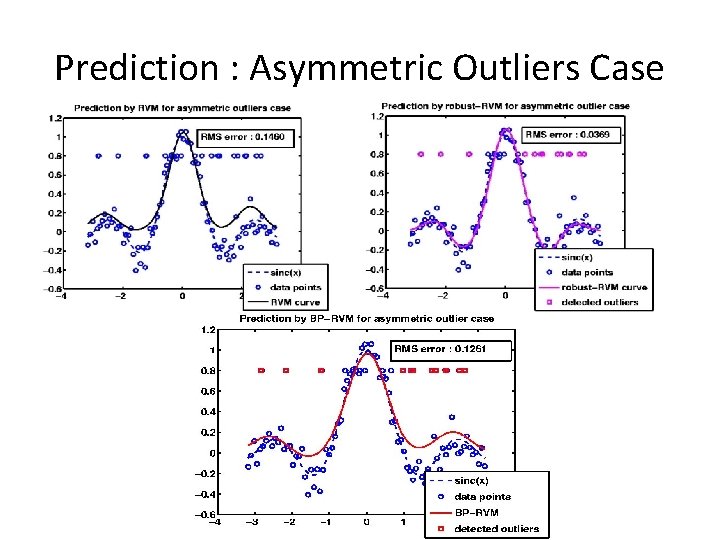
Prediction : Asymmetric Outliers Case

Image Denoising • Salt and pepper noise – Outliers • Regression formulation – Image as a surface over 2 D grid • y: Intensity • x: 2 D grid • Denoised image obtained by prediction

Salt and Pepper Noise

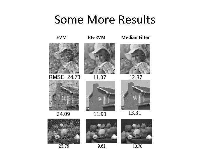
Some More Results RVM RB-RVM Median Filter

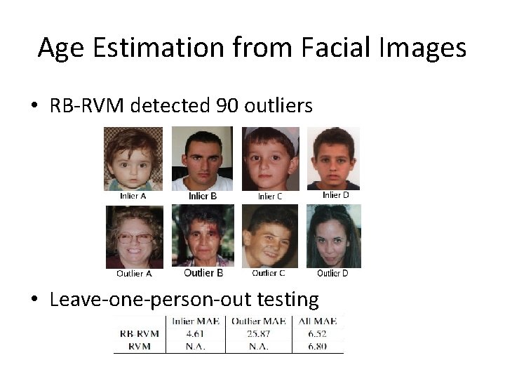
Age Estimation from Facial Images • RB-RVM detected 90 outliers • Leave-one-person-out testing

Summary for Robust RVM • Modeled outliers as sparse variables • Jointly estimated parameter and outliers • Bayesian approach gives very good result

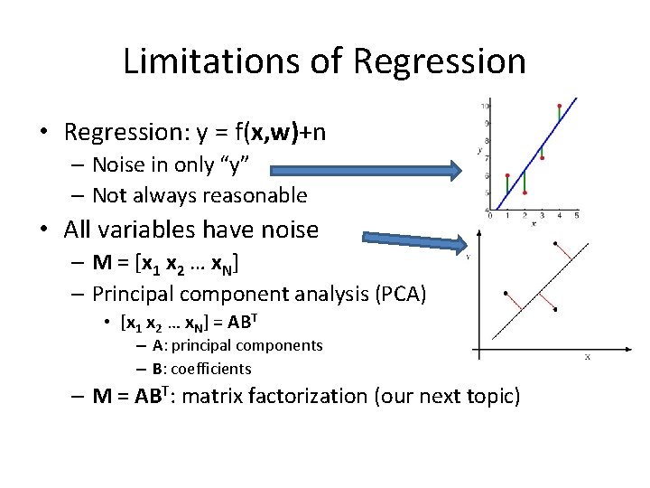
Limitations of Regression • Regression: y = f(x, w)+n – Noise in only “y” – Not always reasonable • All variables have noise – M = [x 1 x 2 … x. N] – Principal component analysis (PCA) • [x 1 x 2 … x. N] = ABT – A: principal components – B: coefficients – M = ABT: matrix factorization (our next topic)

Matrix Factorization in the presence of Missing Data

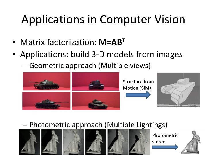
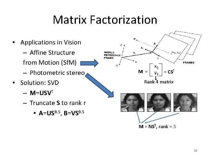
Applications in Computer Vision • Matrix factorization: M=ABT • Applications: build 3 -D models from images – Geometric approach (Multiple views) Structure from Motion (Sf. M) – Photometric approach (Multiple Lightings) Photometric stereo 37

Matrix Factorization • Applications in Vision – Affine Structure from Motion (Sf. M) – Photometric stereo • Solution: SVD – M=USVT – Truncate S to rank r • A=US 0. 5, B=VS 0. 5 M = xij yij = CST Rank 4 matrix M = NST, rank = 3 38

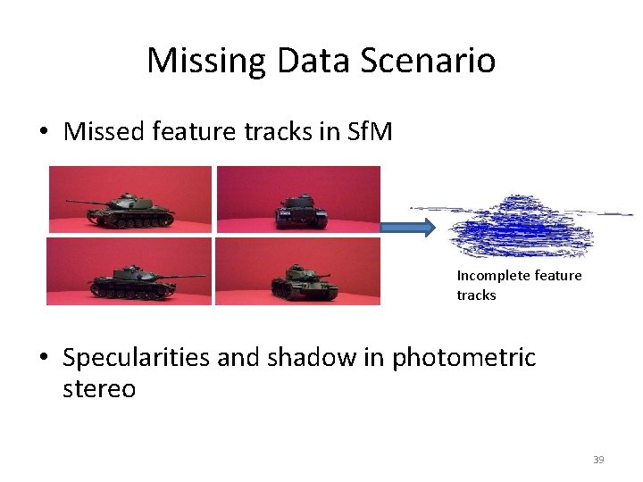
Missing Data Scenario • Missed feature tracks in Sf. M Incomplete feature tracks • Specularities and shadow in photometric stereo 39

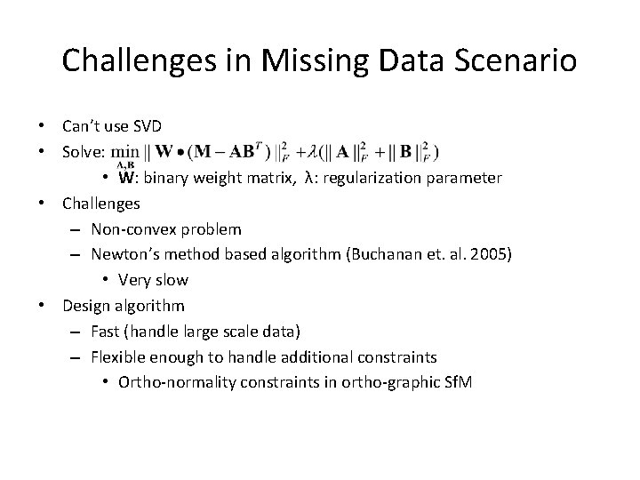
Challenges in Missing Data Scenario • Can’t use SVD • Solve: • W: binary weight matrix, λ: regularization parameter • Challenges – Non-convex problem – Newton’s method based algorithm (Buchanan et. al. 2005) • Very slow • Design algorithm – Fast (handle large scale data) – Flexible enough to handle additional constraints • Ortho-normality constraints in ortho-graphic Sf. M

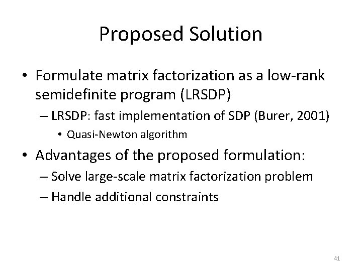
Proposed Solution • Formulate matrix factorization as a low-rank semidefinite program (LRSDP) – LRSDP: fast implementation of SDP (Burer, 2001) • Quasi-Newton algorithm • Advantages of the proposed formulation: – Solve large-scale matrix factorization problem – Handle additional constraints 41

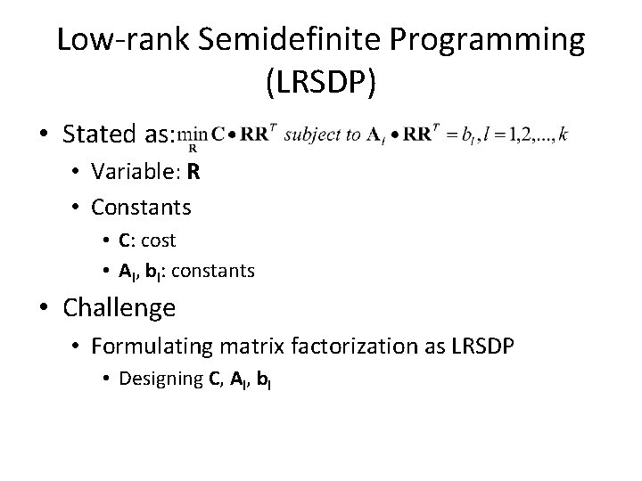
Low-rank Semidefinite Programming (LRSDP) • Stated as: • Variable: R • Constants • C: cost • Al, bl: constants • Challenge • Formulating matrix factorization as LRSDP • Designing C, Al, bl

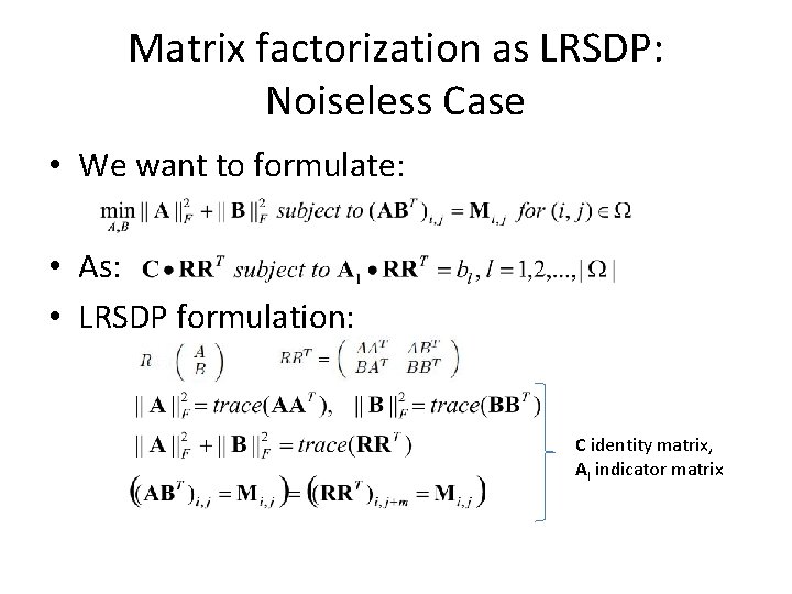
Matrix factorization as LRSDP: Noiseless Case • We want to formulate: • As: • LRSDP formulation: C identity matrix, Al indicator matrix

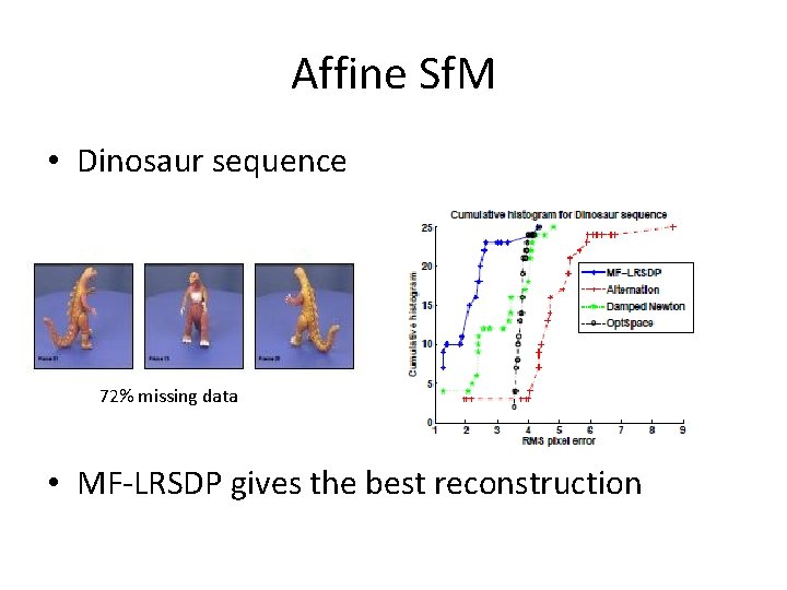
Affine Sf. M • Dinosaur sequence 72% missing data • MF-LRSDP gives the best reconstruction

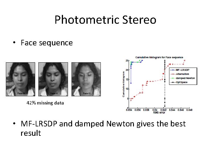
Photometric Stereo • Face sequence 42% missing data • MF-LRSDP and damped Newton gives the best result

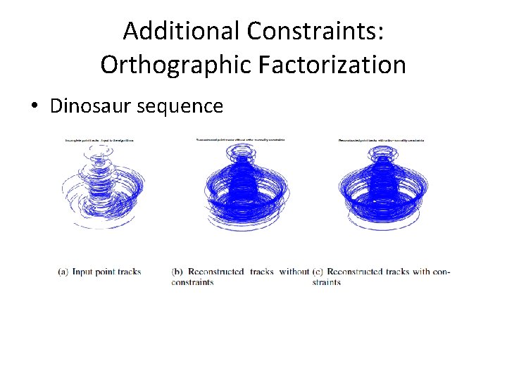
Additional Constraints: Orthographic Factorization • Dinosaur sequence

Summary • Formulated missing data matrix factorization as LRSDP – Large scale problems – Handle additional constraints • Overall summary – Two statistical data models • Regression in presence of outliers – Role of sparsity • Matrix factorization in presence of missing data – Low rank semidefinite program

Thank you! Questions? 48