Great Theoretical Ideas In Computer Science Victor Adamchik

Great Theoretical Ideas In Computer Science Victor Adamchik Lecture 8 CS 15 -251 Graphs - I Carnegie Mellon University

Plan Graph Representations Counting Trees Cayley’s Formula Prϋfer Sequence Minimum Spanning Trees Planar Graphs Euler’s Polyhedra Theorem

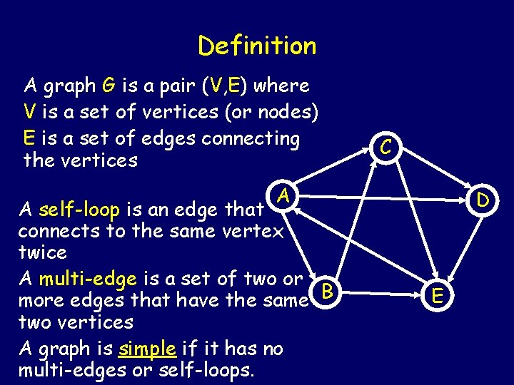
Definition A graph G is a pair (V, E) where V is a set of vertices (or nodes) E is a set of edges connecting the vertices C A A self-loop is an edge that connects to the same vertex twice A multi-edge is a set of two or more edges that have the same B two vertices A graph is simple if it has no multi-edges or self-loops. D E

More terms Directed: an edge is an ordered pair of vertices Undirected: edge is unordered pair of vertices Weighted: (a cost associated with an edge) Path (is a sequence of vertices) Cycle (the start and end vertices are the same) Acyclic Connected or Disconnected The degree of a vertex (in an undirected graph is the number of edges associated with it. )

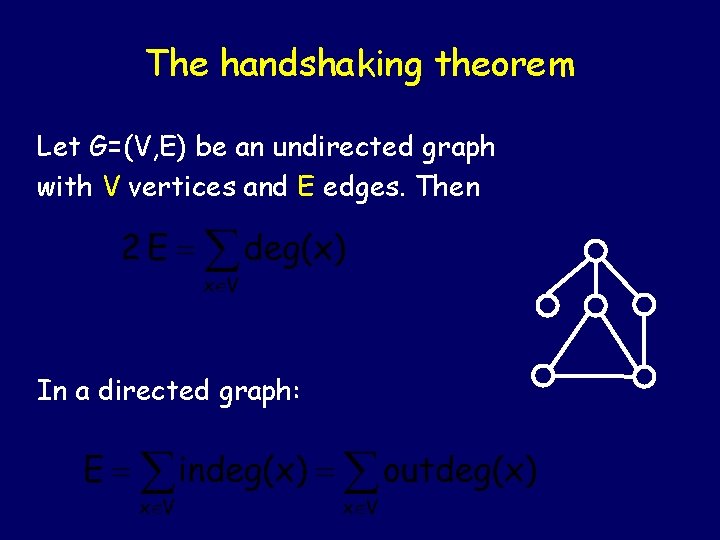
The handshaking theorem Let G=(V, E) be an undirected graph with V vertices and E edges. Then In a directed graph:

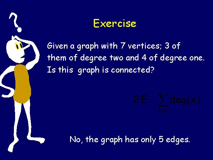
Exercise Given a graph with 7 vertices; 3 of them of degree two and 4 of degree one. Is this graph is connected? No, the graph has only 5 edges.

Representing Graphs Adjacency List or Adjacency Matrix Vertex X is adjacent to vertex Y if and only if there is an edge (X, Y) between them.

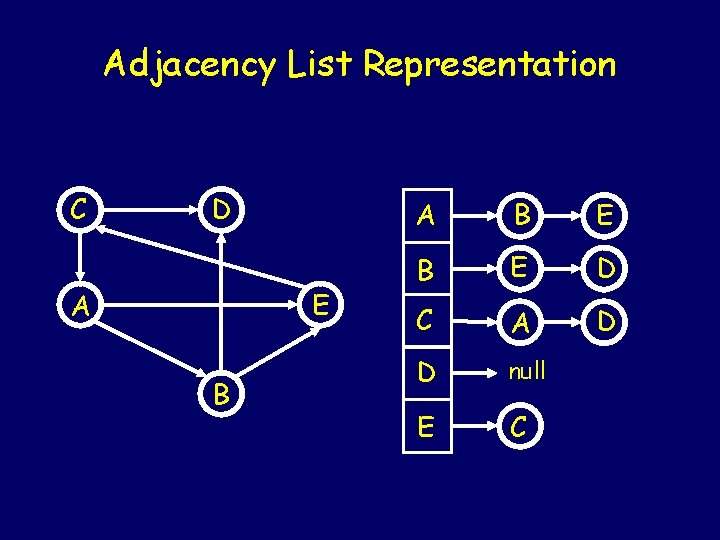
Adjacency List Representation C D E A B E B E D C A D D null E C

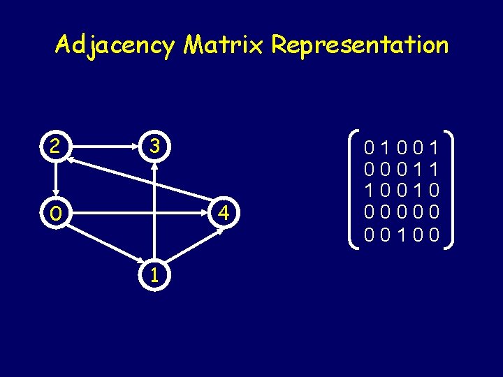
Adjacency Matrix Representation 2 3 4 0 1 01001 00011 10010 00000 00100

Representing Graphs Adjacency List Representation is used for representation of the sparse graphs. Adjacency Matrix Representation is used for representation of the dense graphs.

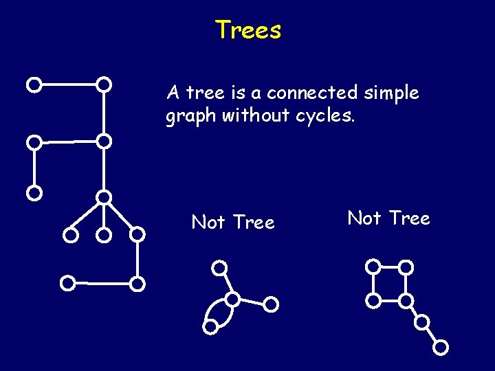
Trees A tree is a connected simple graph without cycles. Not Tree

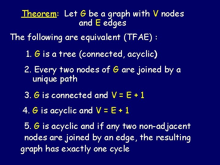
Theorem: Let G be a graph with V nodes and E edges The following are equivalent (TFAE) : 1. G is a tree (connected, acyclic) 2. Every two nodes of G are joined by a unique path 3. G is connected and V = E + 1 4. G is acyclic and V = E + 1 5. G is acyclic and if any two non-adjacent nodes are joined by an edge, the resulting graph has exactly one cycle

To prove this, it suffices to show 1 2 3 4 5 1 We’ll just show 1 2 3 4 and leave the rest to the reader

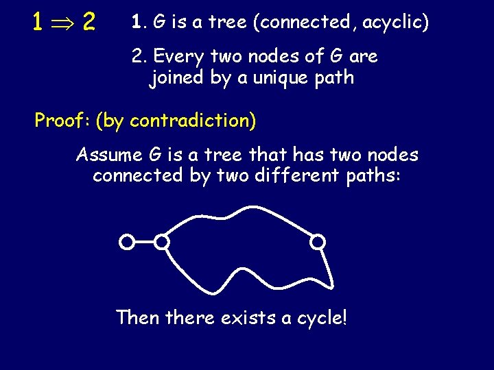
1 2 1. G is a tree (connected, acyclic) 2. Every two nodes of G are joined by a unique path Proof: (by contradiction) Assume G is a tree that has two nodes connected by two different paths: Then there exists a cycle!

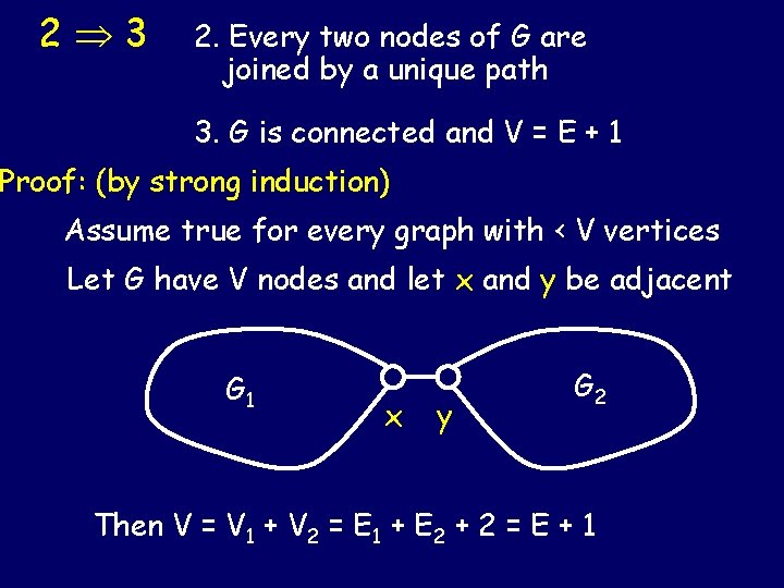
2 3 2. Every two nodes of G are joined by a unique path 3. G is connected and V = E + 1 Proof: (by strong induction) Assume true for every graph with < V vertices Let G have V nodes and let x and y be adjacent G 1 x y G 2 Then V = V 1 + V 2 = E 1 + E 2 + 2 = E + 1

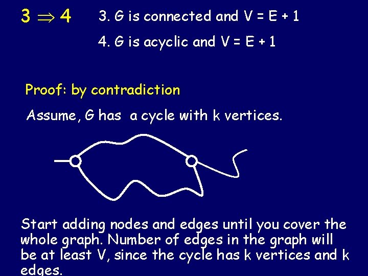
3 4 3. G is connected and V = E + 1 4. G is acyclic and V = E + 1 Proof: by contradiction Assume, G has a cycle with k vertices. Start adding nodes and edges until you cover the whole graph. Number of edges in the graph will be at least V, since the cycle has k vertices and k edges.

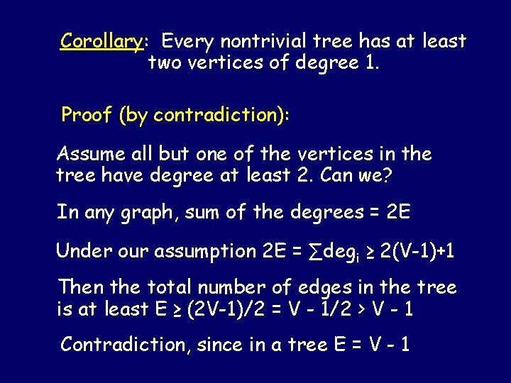
Corollary: Every nontrivial tree has at least two vertices of degree 1. Proof (by contradiction): Assume all but one of the vertices in the tree have degree at least 2. Can we? In any graph, sum of the degrees = 2 E Under our assumption 2 E = ∑degi ≥ 2(V-1)+1 Then the total number of edges in the tree is at least E ≥ (2 V-1)/2 = V - 1/2 > V - 1 Contradiction, since in a tree E = V - 1

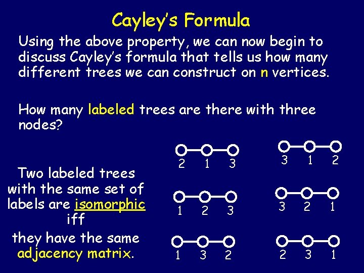
Cayley’s Formula Using the above property, we can now begin to discuss Cayley’s formula that tells us how many different trees we can construct on n vertices. How many labeled trees are there with three nodes? Two labeled trees with the same set of labels are isomorphic iff they have the same adjacency matrix. 2 1 3 3 1 2 3 3 2 1 1 3 2 2 3 1

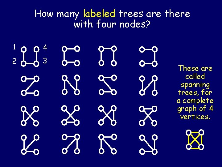
How many labeled trees are there with four nodes? 1 4 2 3 These are called spanning trees, for a complete graph of 4 vertices.

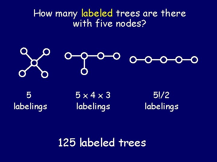
How many labeled trees are there with five nodes? 5 labelings 5 x 4 x 3 labelings 5!/2 labelings 125 labeled trees

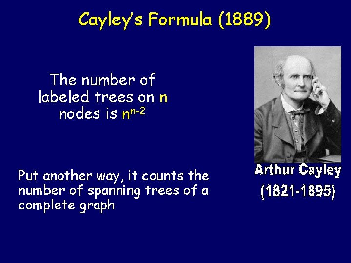
Cayley’s Formula (1889) The number of labeled trees on n nodes is nn-2 Put another way, it counts the number of spanning trees of a complete graph

Prϋfer Encoding (1918) We are going to find a bijection between the set of sequences and the set of labeled trees. A Prϋfer sequence is a sequence of n− 2 numbers, each being one of the numbers 1 through n. We should initially note that indeed there are nn− 2 Prϋfer sequences for any given n. bijection: T(n) -> P(n-2)

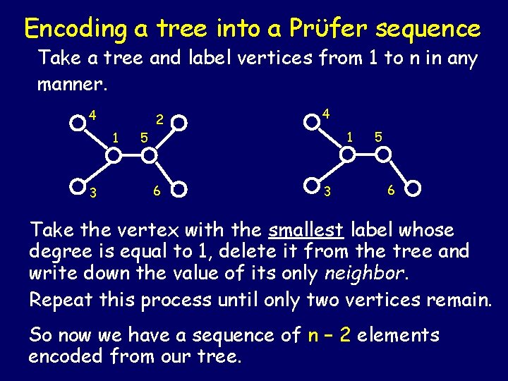
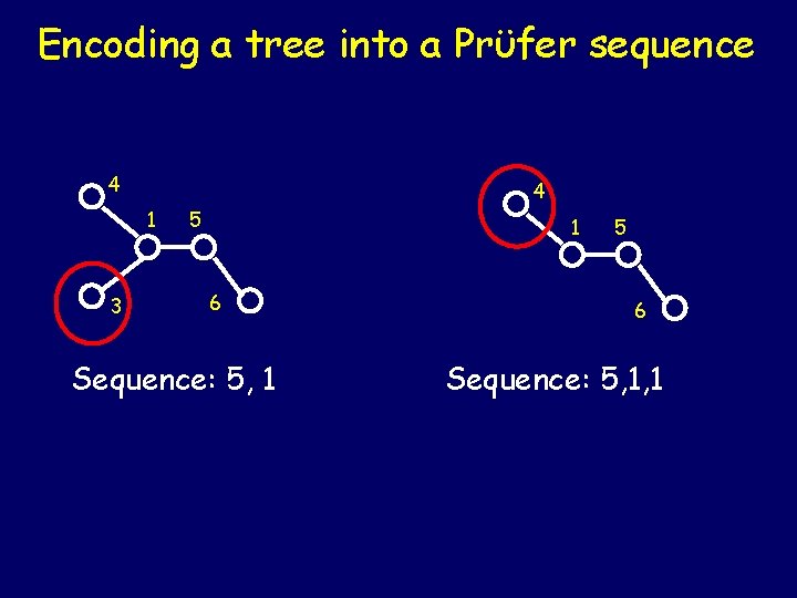
Encoding a tree into a Prϋfer sequence Take a tree and label vertices from 1 to n in any manner. 4 1 3 2 4 6 3 1 5 5 6 Take the vertex with the smallest label whose degree is equal to 1, delete it from the tree and write down the value of its only neighbor. Repeat this process until only two vertices remain. So now we have a sequence of n − 2 elements encoded from our tree.

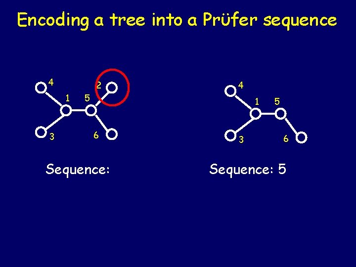
Encoding a tree into a Prϋfer sequence 4 2 1 3 4 5 1 6 Sequence: 3 5 6 Sequence: 5

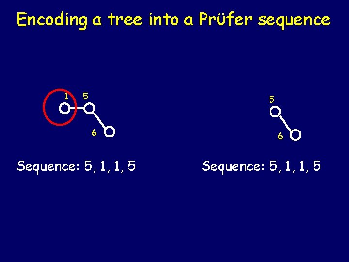
Encoding a tree into a Prϋfer sequence 4 4 1 3 5 1 6 Sequence: 5, 1 5 6 Sequence: 5, 1, 1

Encoding a tree into a Prϋfer sequence 1 5 5 6 Sequence: 5, 1, 1, 5

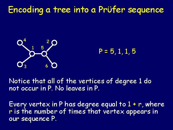
Encoding a tree into a Prϋfer sequence 4 2 1 3 5 P = 5, 1, 1, 5 6 Notice that all of the vertices of degree 1 do not occur in P. No leaves in P. Every vertex in P has degree equal to 1 + r, where r is the number of times that vertex appears in our sequence P.

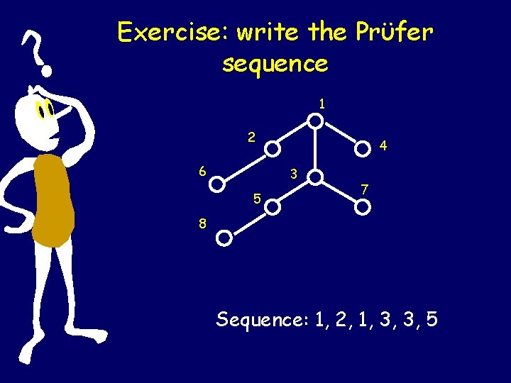
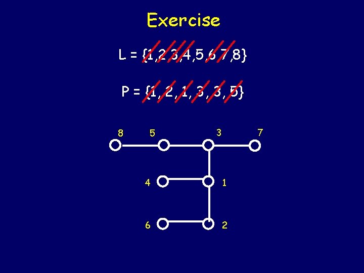
Exercise: write the Prϋfer sequence 1 2 6 4 3 5 7 8 Sequence: 1, 2, 1, 3, 3, 5

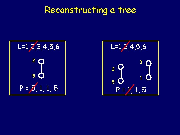
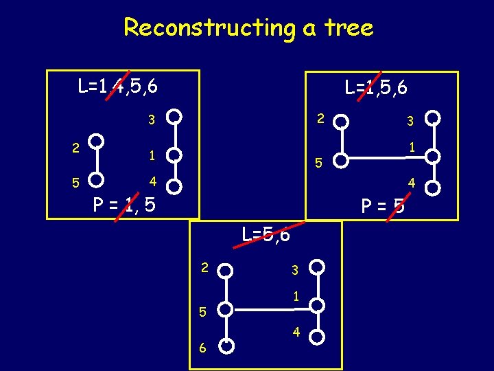
Reconstructing a tree Given P = {a 1, …, an-2} and the list L = {1, …, n} Let k be the smallest number in L that is not in P. Let aj be the fist number in the Prϋfer sequence P. Connect k and aj with an edge. Remove k from L and aj from P. Repeat this process until all elements of P have been exhausting (n-2 times) Connect the last two vertices in L with an edge.

Reconstructing a tree L=1, 2, 3, 4, 5, 6 L=1, 3, 4, 5, 6 2 3 2 5 P = 5, 1, 1, 5 5 1 P = 1, 1, 5

Reconstructing a tree L=1, 4, 5, 6 L=1, 5, 6 2 3 2 5 1 3 1 5 4 4 P = 1, 5 P=5 L=5, 6 2 5 6 3 1 4

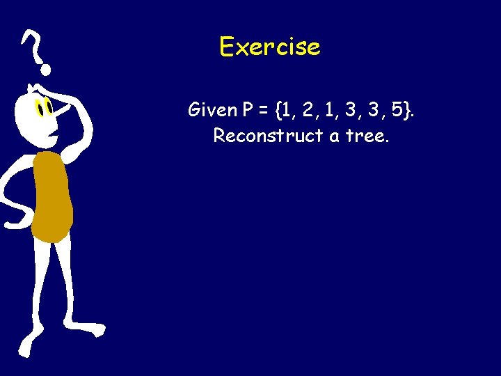
Exercise Given P = {1, 2, 1, 3, 3, 5}. Reconstruct a tree.

Exercise L = {1, 2, 3, 4, 5, 6, 7, 8} P = {1, 2, 1, 3, 3, 5} 8 5 3 7 4 1 6 2

Bijection between Prüfer Sequences and Labeled Trees Let T be a set of labeled tree of n vertices Let P be a set of Prüfer sequences of length n-2 A map f: T-> P is a bijection.

A map f: T-> P is injective. We need to show that two different trees T 1 , T 2 generate different Prϋfer sequences. By Induction on the number of vertices. Base case: n = 2, two vertices joined by an edge. Assume it’s true for n, prove it for n+1. Take the lowest-labeled leaf in T 1 and in T 2. Case 1: Those two leaves are different Case 2: Same, but neighbors not Case 3: Leaves and neighbors are the same

A map f: T-> P is surjective. We need to show that any sequence P={a 1, …, an-2} generates at least one tree on L={1, …, n} By Induction on the number of vertices. Base case: n = 2, P = {}. Assume it’s true for n, prove it for n+1. Take the lowest vk L s. t. vk P Consider P’=Pa 1 and L’= Lvk. By IH there is T’. Form T from T’ by adding vk joined with a 1. Since a 1 is internal, T is a tree.

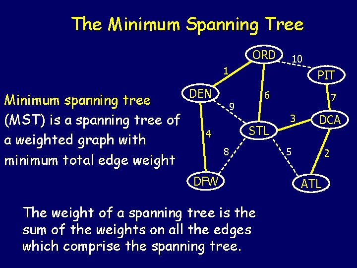
The Minimum Spanning Tree ORD 10 1 DEN Minimum spanning tree (MST) is a spanning tree of 4 a weighted graph with minimum total edge weight PIT 6 9 STL 8 DFW The weight of a spanning tree is the sum of the weights on all the edges which comprise the spanning tree. 7 3 DCA 5 2 ATL

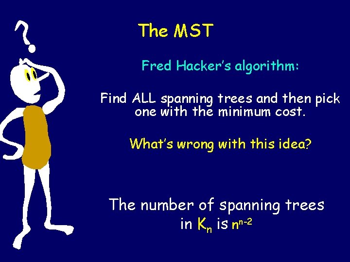
The MST Fred Hacker’s algorithm: Find ALL spanning trees and then pick one with the minimum cost. What’s wrong with this idea? The number of spanning trees in Kn is nn-2

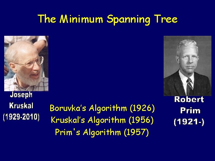
The Minimum Spanning Tree Boruvka’s Algorithm (1926) Kruskal’s Algorithm (1956) Prim's Algorithm (1957)

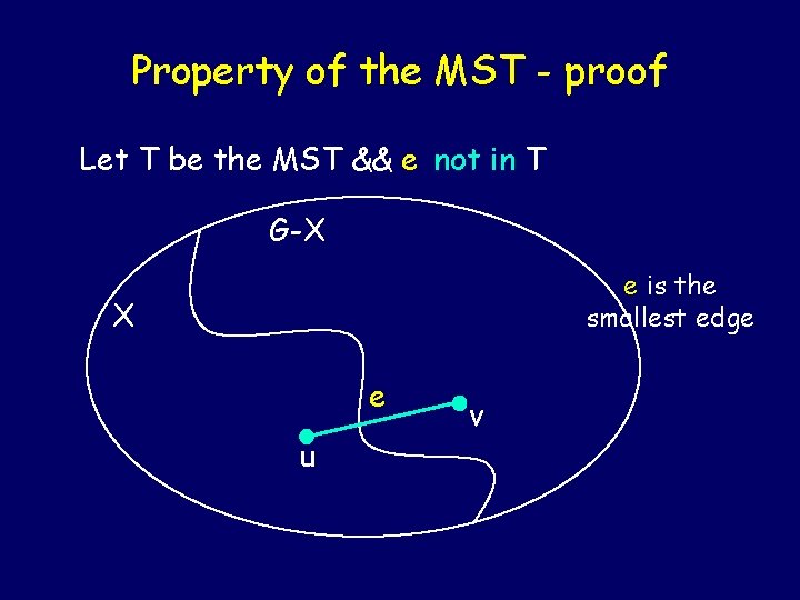
Property of the MST Lemma: Let X be any subset of the vertices of G, and let edge e be the smallest edge connecting X to G-X. Then e is part of the minimum spanning tree.

Property of the MST - proof Let T be the MST && e not in T G-X e is the smallest edge X e u v

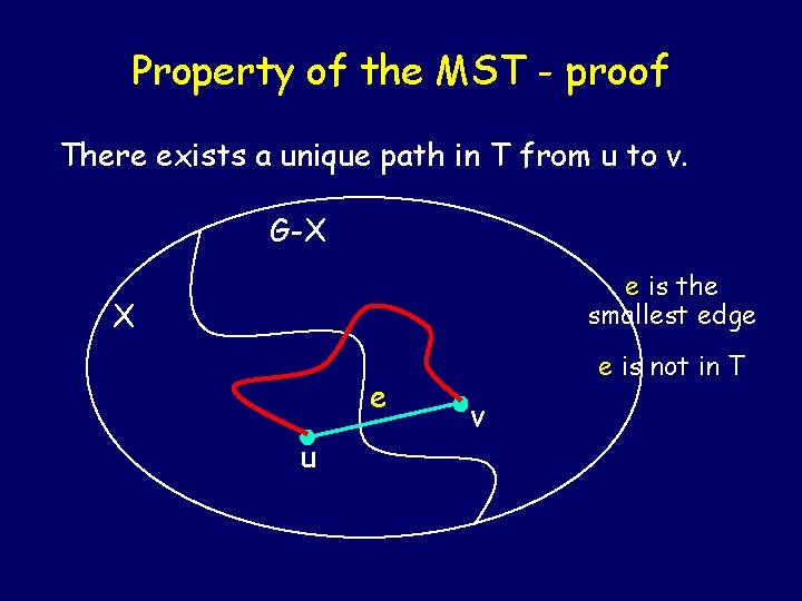
Property of the MST - proof There exists a unique path in T from u to v. G-X e is the smallest edge X e u e is not in T v

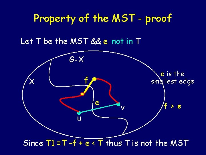
Property of the MST - proof Let T be the MST && e not in T G-X e is the smallest edge f X e u v f > e Since T 1 =T –f + e < T thus T is not the MST

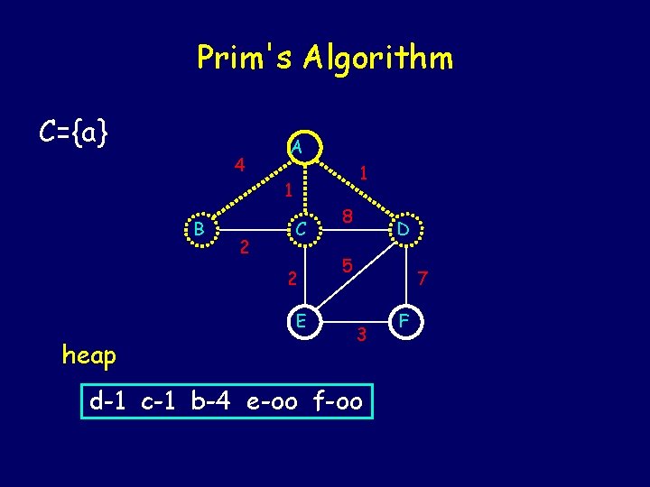
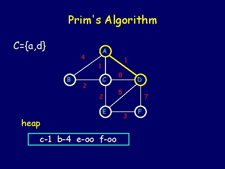
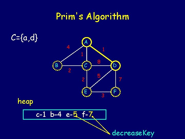
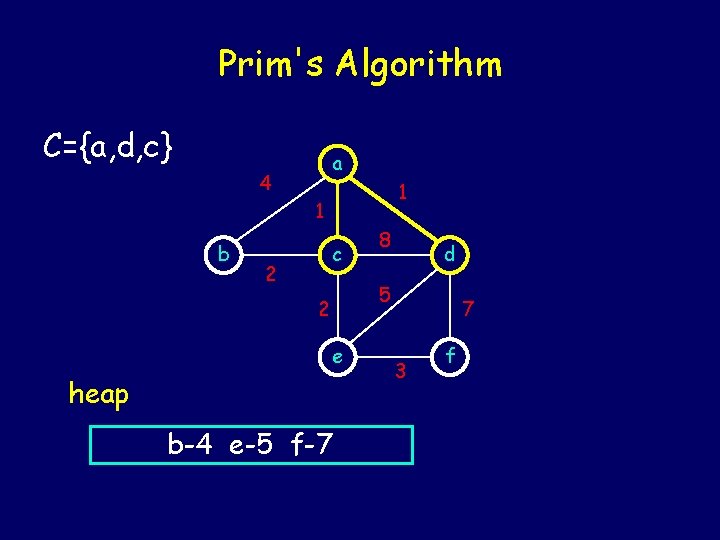
Prim's Algorithm algorithm builds a tree one VERTEX at a time. - Start with an arbitrary vertex as component C - Expand C by adding a vertex having the minimum weight edge of the graph having exactly one end point in C. - Continue to grow the tree until C gets all vertices.

Prim's Algorithm C={a} 4 A 1 1 B 2 C 2 E heap 8 D 5 7 3 d-1 c-1 b-4 e-oo f-oo F

Prim's Algorithm C={a, d} A 4 1 1 B 2 C 2 E heap c-1 b-4 e-oo f-oo 8 D 5 7 3 F

Prim's Algorithm C={a, d} A 4 1 1 B 2 C 2 E heap 8 D 5 7 3 F c-1 b-4 e-5 f-7 decrease. Key

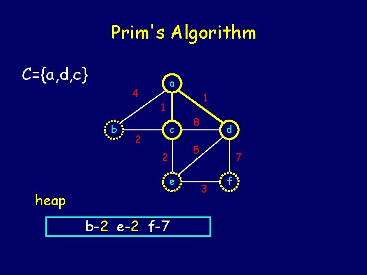
Prim's Algorithm C={a, d, c} a 4 1 1 b c 2 8 d 5 2 e heap b-4 e-5 f-7 7 3 f

Prim's Algorithm C={a, d, c} a 4 1 1 b c 2 8 d 5 2 e heap b-2 e-2 f-7 7 3 f

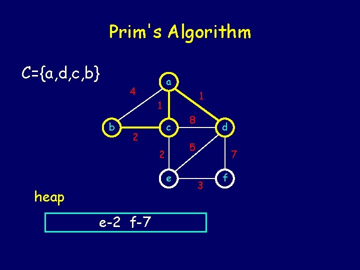
Prim's Algorithm C={a, d, c, b} a 4 1 1 b c 2 e e-2 f-7 d 5 2 heap 8 7 3 f

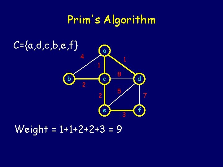
Prim's Algorithm C={a, d, c, b, e, f} a 4 1 1 b c 2 8 d 5 2 e 7 3 Weight = 1+1+2+2+3 = 9 f

What is the worst-case runtime complexity of Prim's Algorithm? We maintain a PQ of vertices: We run delete. Min V times We update the queue E times O(V*log V + E*log V)

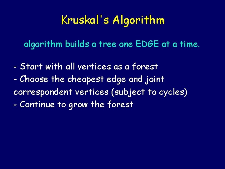
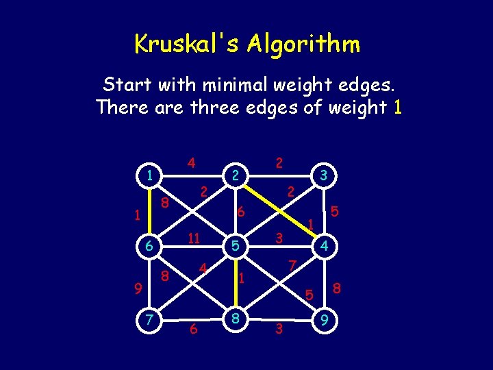
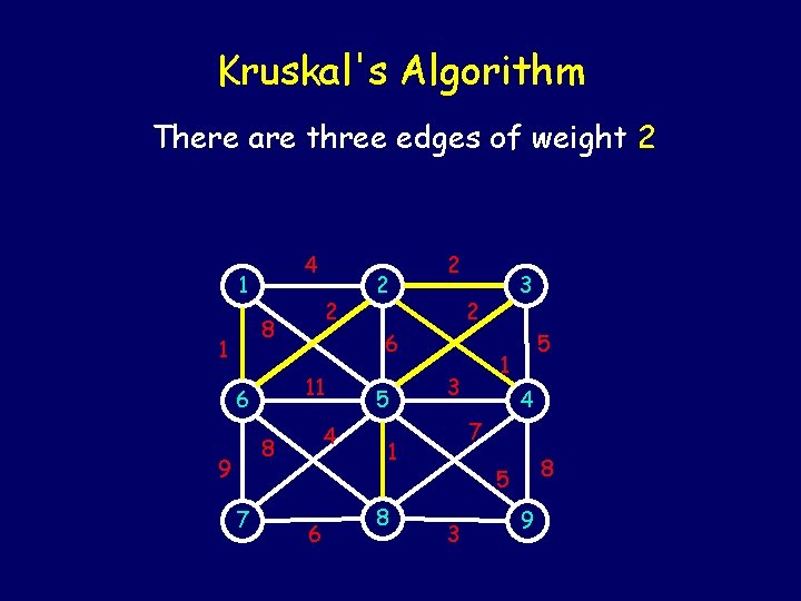
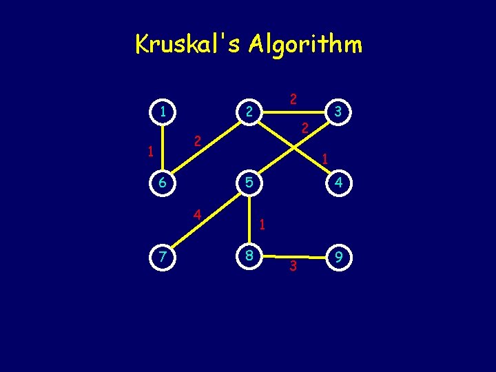
Kruskal's Algorithm algorithm builds a tree one EDGE at a time. - Start with all vertices as a forest - Choose the cheapest edge and joint correspondent vertices (subject to cycles) - Continue to grow the forest

Kruskal's Algorithm Start with minimal weight edges. There are three edges of weight 1 4 1 2 8 1 4 8 9 7 6 5 5 1 3 4 7 1 8 3 2 6 11 6 2 2 8 5 3 9

Kruskal's Algorithm There are three edges of weight 2 4 1 2 8 1 4 8 9 7 6 5 5 1 3 4 7 1 8 3 2 6 11 6 2 2 8 5 3 9

Kruskal's Algorithm 1 2 2 1 6 1 5 4 7 3 4 1 8 3 9

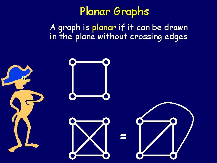
Planar Graphs A graph is planar if it can be drawn in the plane without crossing edges =

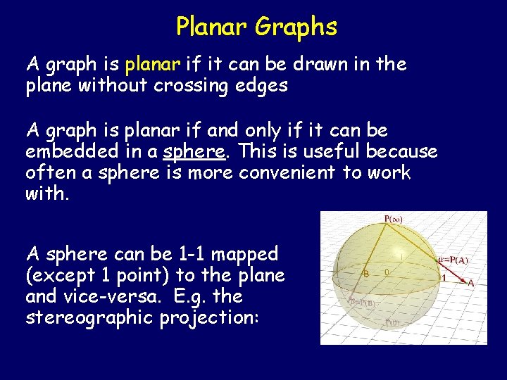
Planar Graphs A graph is planar if it can be drawn in the plane without crossing edges A graph is planar if and only if it can be embedded in a sphere. This is useful because often a sphere is more convenient to work with. A sphere can be 1 -1 mapped (except 1 point) to the plane and vice-versa. E. g. the stereographic projection:

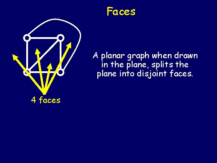
Faces A planar graph when drawn in the plane, splits the plane into disjoint faces. 4 faces

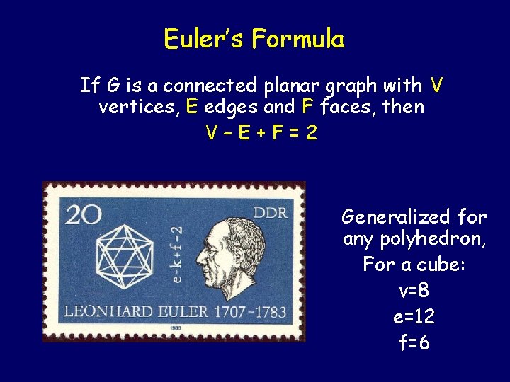
Euler’s Formula If G is a connected planar graph with V vertices, E edges and F faces, then V–E+F=2 Generalized for any polyhedron, For a cube: v=8 e=12 f=6

Proof of Euler’s Formula For connected arbitrary planar graphs V – E + F = 2 The proof is by induction on edges. Start with a single edge and 2 vertices: V=2, E=1, F=1. Check. Add the edges in an order so that we’ve added so far is connected. There are two cases to consider.

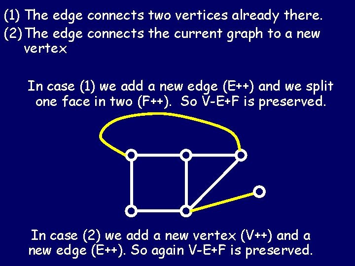
(1) The edge connects two vertices already there. (2) The edge connects the current graph to a new vertex In case (1) we add a new edge (E++) and we split one face in two (F++). So V-E+F is preserved. In case (2) we add a new vertex (V++) and a new edge (E++). So again V-E+F is preserved.

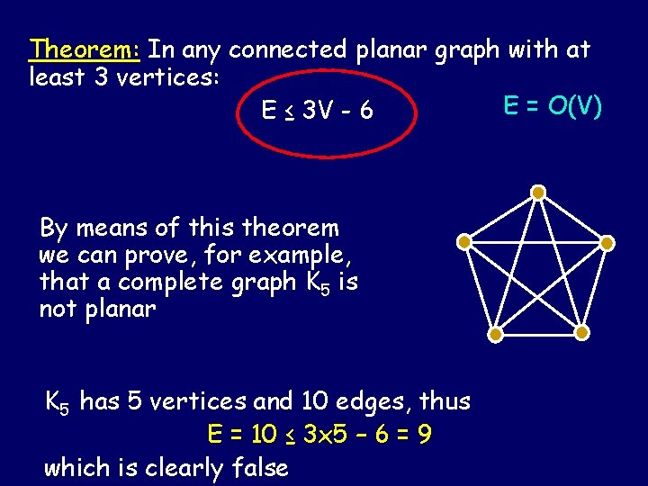
Theorem: In any connected planar graph with at least 3 vertices: E = O(V) E ≤ 3 V - 6 By means of this theorem we can prove, for example, that a complete graph K 5 is not planar K 5 has 5 vertices and 10 edges, thus E = 10 ≤ 3 x 5 – 6 = 9 which is clearly false

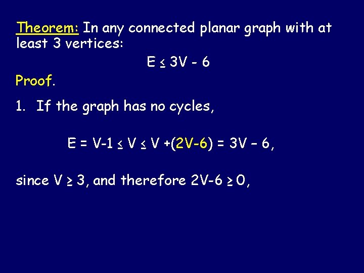
Theorem: In any connected planar graph with at least 3 vertices: E ≤ 3 V - 6 Proof. 1. If the graph has no cycles, E = V-1 ≤ V +(2 V-6) = 3 V – 6, since V ≥ 3, and therefore 2 V-6 ≥ 0,

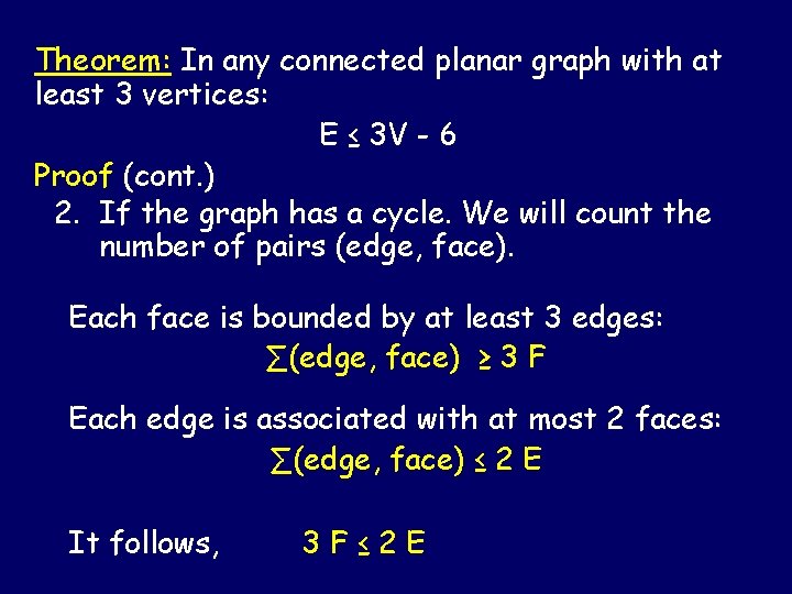
Theorem: In any connected planar graph with at least 3 vertices: E ≤ 3 V - 6 Proof (cont. ) 2. If the graph has a cycle. We will count the number of pairs (edge, face). Each face is bounded by at least 3 edges: ∑(edge, face) ≥ 3 F Each edge is associated with at most 2 faces: ∑(edge, face) ≤ 2 E It follows, 3 F≤ 2 E

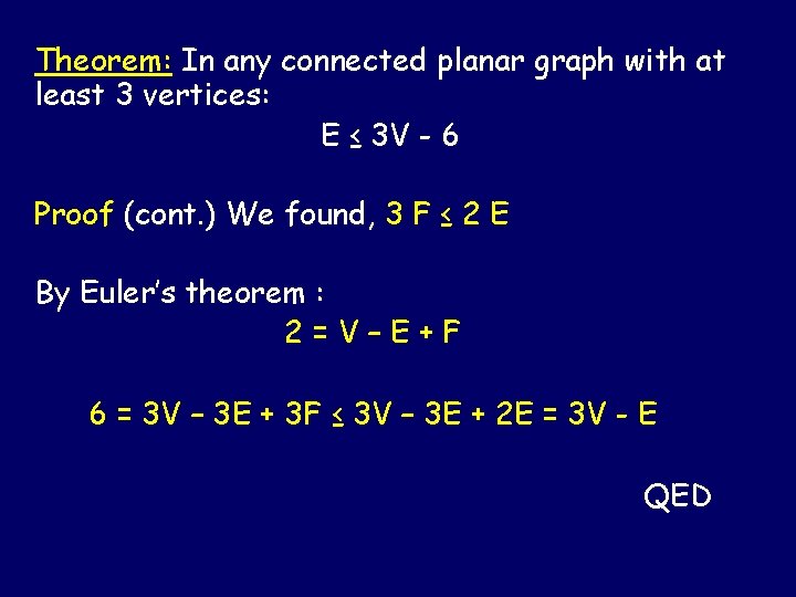
Theorem: In any connected planar graph with at least 3 vertices: E ≤ 3 V - 6 Proof (cont. ) We found, 3 F ≤ 2 E By Euler’s theorem : 2=V–E+F 6 = 3 V – 3 E + 3 F ≤ 3 V – 3 E + 2 E = 3 V - E QED

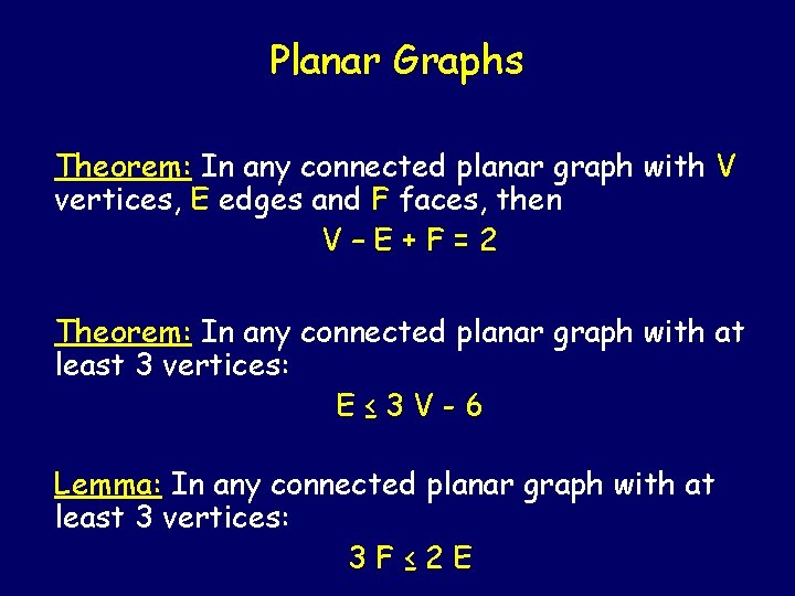
Planar Graphs Theorem: In any connected planar graph with V vertices, E edges and F faces, then V–E+F=2 Theorem: In any connected planar graph with at least 3 vertices: E≤ 3 V-6 Lemma: In any connected planar graph with at least 3 vertices: 3 F≤ 2 E

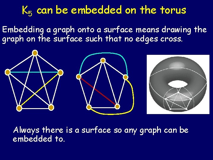
K 5 can be embedded on the torus Embedding a graph onto a surface means drawing the graph on the surface such that no edges cross. Always there is a surface so any graph can be embedded to.

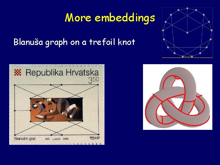
More embeddings Blanuša graph on a trefoil knot

Cayley’s Formula Prϋfer Encoding Minimum Spanning Trees Planar Graphs Euler’s Polyhedra Theorem Here’s What You Need to Know…