Flow tracing and watershed analysis Geospatial Analysis and

Flow tracing and watershed analysis Geospatial Analysis and Modeling: Lecture notes Helena Mitasova, NCSU MEAS

Outline • cumulative terrain parameters based on flow tracing: flow path length, flow accumulation, • methods for computing flow direction (D*8, Dinf), flow tracing (SFD, MFD, uniform, weighted) • methods for flow tracing through depressions and flat areas • extracting watershed boundaries, computing watershed hierarchies

Cumulative flow parameters Parameters and features: • flow path length, • flow accumulation and stream networks • watersheds and ridge lines Computed using flow lines

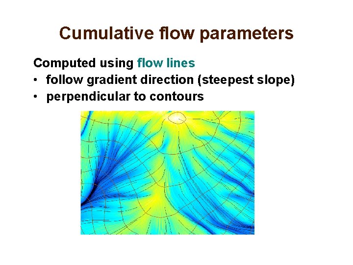
Cumulative flow parameters Computed using flow lines • follow gradient direction (steepest slope) • perpendicular to contours

Computing flow direction What is flow direction? How to compute it? D-8 and D-infinity

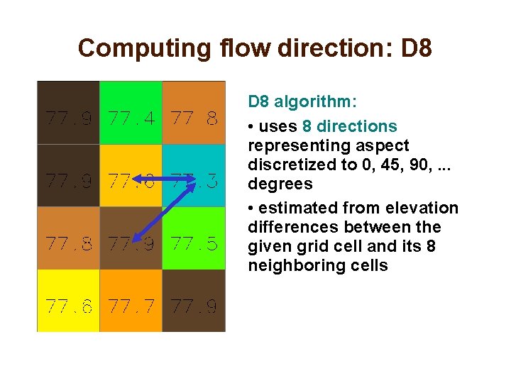
Computing flow direction: D 8 algorithm: • uses 8 directions representing aspect discretized to 0, 45, 90, . . . degrees • estimated from elevation differences between the given grid cell and its 8 neighboring cells

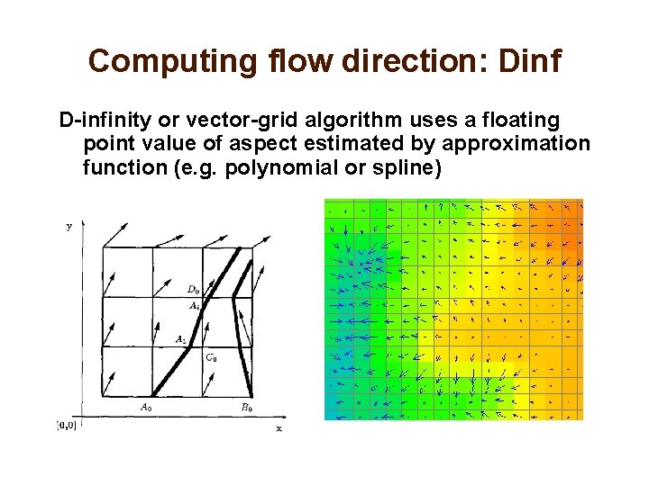
Computing flow direction: Dinf D-infinity or vector-grid algorithm uses a floating point value of aspect estimated by approximation function (e. g. polynomial or spline)

Flow routing Tracing flow in the gradient direction to compute • flow path length • flow accumulation

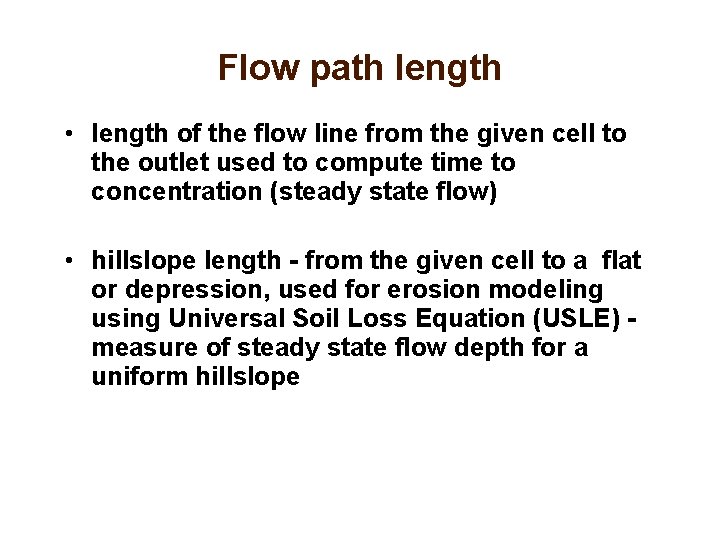
Flow path length • length of the flow line from the given cell to the outlet used to compute time to concentration (steady state flow) • hillslope length - from the given cell to a flat or depression, used for erosion modeling using Universal Soil Loss Equation (USLE) measure of steady state flow depth for a uniform hillslope

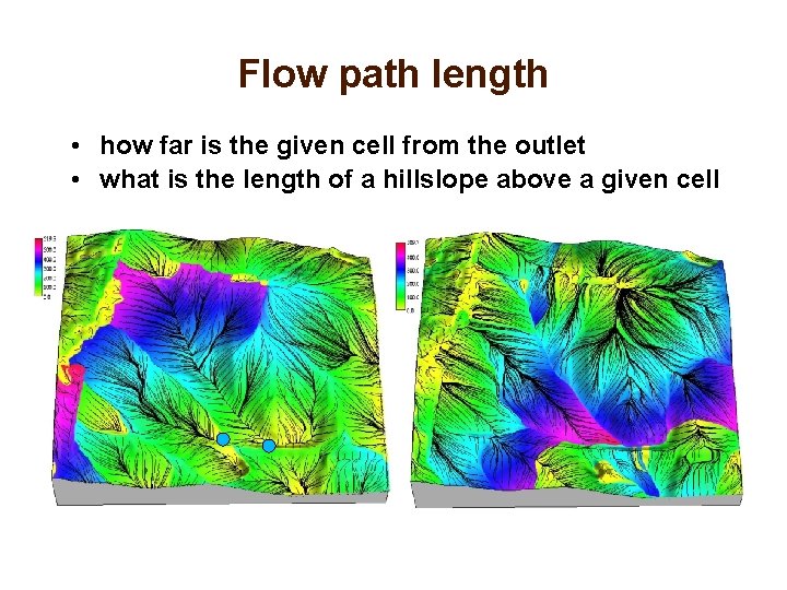
Flow path length • how far is the given cell from the outlet • what is the length of a hillslope above a given cell

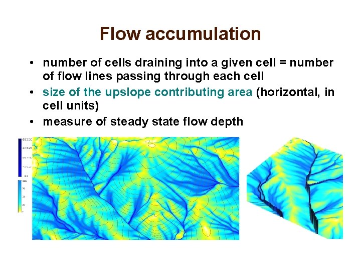
Flow accumulation • number of cells draining into a given cell = number of flow lines passing through each cell • size of the upslope contributing area (horizontal, in cell units) • measure of steady state flow depth

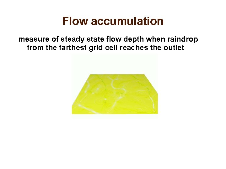
Flow accumulation measure of steady state flow depth when raindrop from the farthest grid cell reaches the outlet

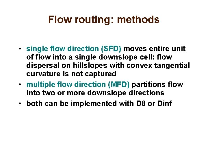
Flow routing: methods • single flow direction (SFD) moves entire unit of flow into a single downslope cell: flow dispersal on hillslopes with convex tangential curvature is not captured • multiple flow direction (MFD) partitions flow into two or more downslope directions • both can be implemented with D 8 or Dinf

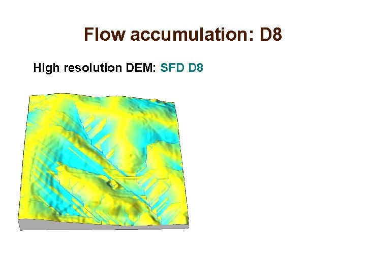
Flow accumulation: D 8 High resolution DEM: SFD D 8

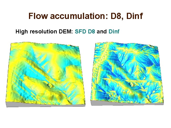
Flow accumulation: D 8, Dinf High resolution DEM: SFD D 8 and Dinf

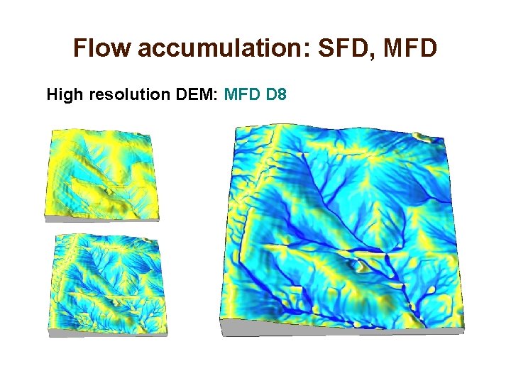
Flow accumulation: SFD, MFD High resolution DEM: MFD D 8

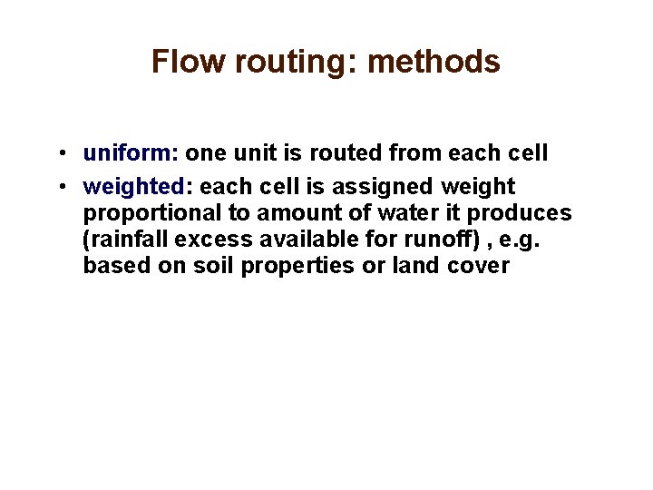
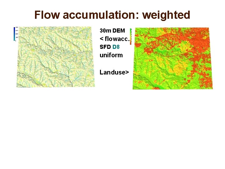
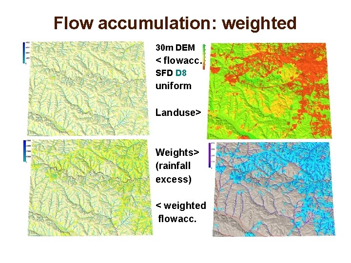
Flow routing: methods • uniform: one unit is routed from each cell • weighted: each cell is assigned weight proportional to amount of water it produces (rainfall excess available for runoff) , e. g. based on soil properties or land cover

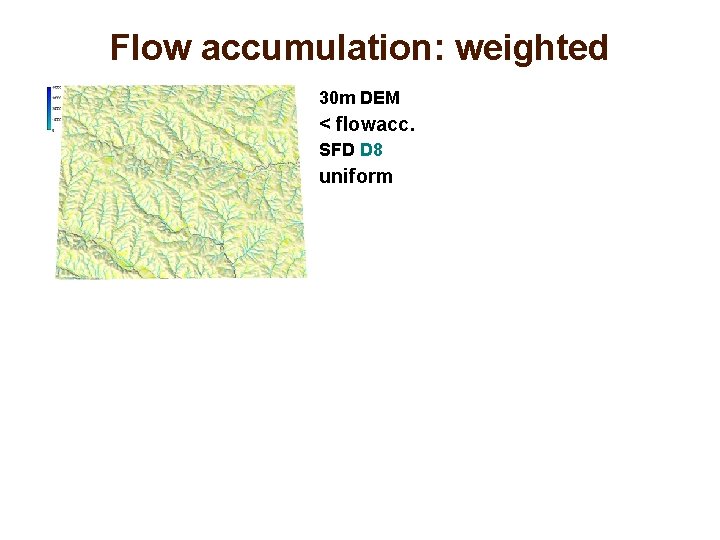
Flow accumulation: weighted 30 m DEM < flowacc. SFD D 8 uniform

Flow accumulation: weighted 30 m DEM < flowacc. SFD D 8 uniform Landuse>

Flow accumulation: weighted 30 m DEM < flowacc. SFD D 8 uniform Landuse> Weights> (rainfall excess) < weighted flowacc.

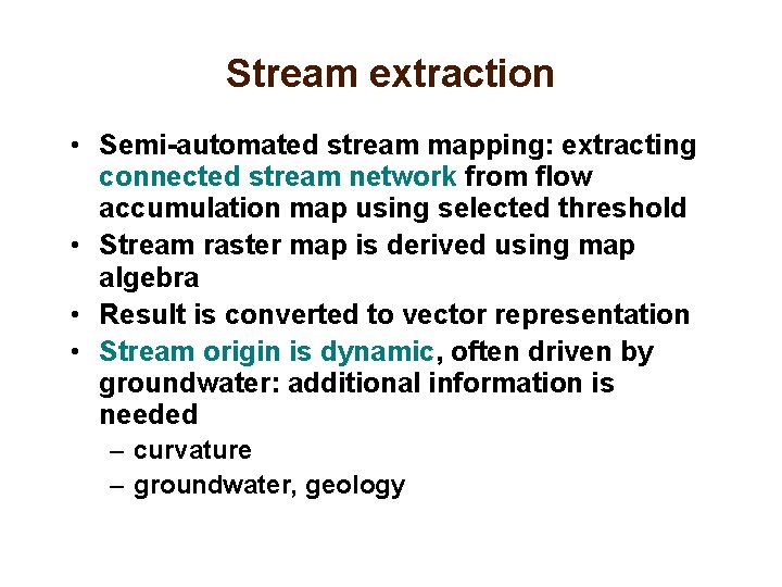
Stream extraction • Semi-automated stream mapping: extracting connected stream network from flow accumulation map using selected threshold • Stream raster map is derived using map algebra • Result is converted to vector representation • Stream origin is dynamic, often driven by groundwater: additional information is needed – curvature – groundwater, geology

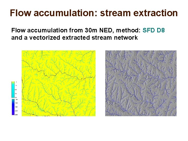
Flow accumulation: stream extraction Flow accumulation from 30 m NED, method: SFD D 8 and a vectorized extracted stream network

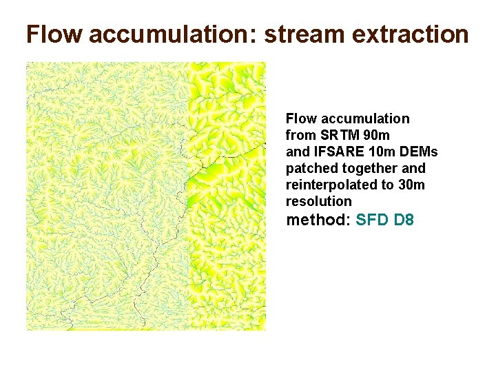
Flow accumulation: stream extraction Flow accumulation from SRTM 90 m and IFSARE 10 m DEMs patched together and reinterpolated to 30 m resolution method: SFD D 8

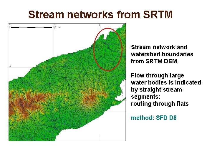
Stream networks from SRTM Stream network and watershed boundaries from SRTM DEM Flow through large water bodies is indicated by straight stream segments: routing through flats method: SFD D 8

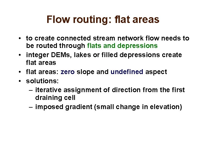
Flow routing: flat areas • to create connected stream network flow needs to be routed through flats and depressions • integer DEMs, lakes or filled depressions create flat areas • flat areas: zero slope and undefined aspect • solutions: – iterative assignment of direction from the first draining cell – imposed gradient (small change in elevation)

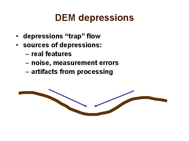
DEM depressions • depressions “trap” flow • sources of depressions: – real features – noise, measurement errors – artifacts from processing

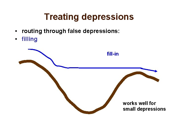
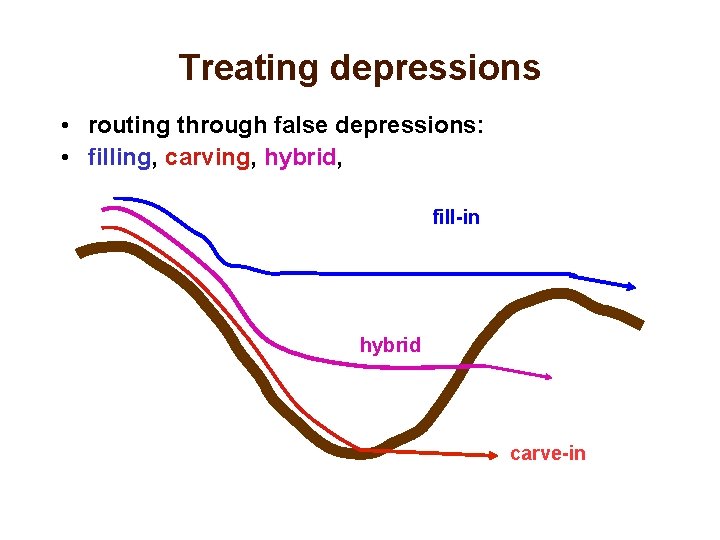
Treating depressions • routing through false depressions: • filling fill-in works well for small depressions

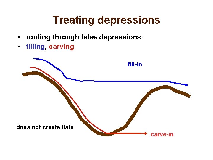
Treating depressions • routing through false depressions: • filling, carving fill-in does not create flats carve-in

Treating depressions • routing through false depressions: • filling, carving, hybrid, fill-in hybrid carve-in

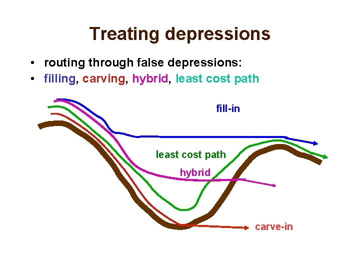
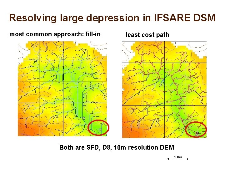
Treating depressions • routing through false depressions: • filling, carving, hybrid, least cost path fill-in least cost path hybrid carve-in

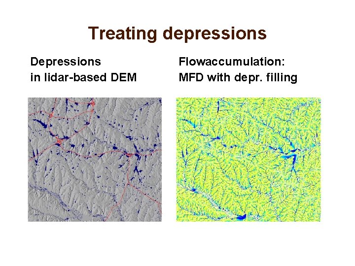
Treating depressions Depressions in lidar-based DEM Flowaccumulation: MFD with depr. filling

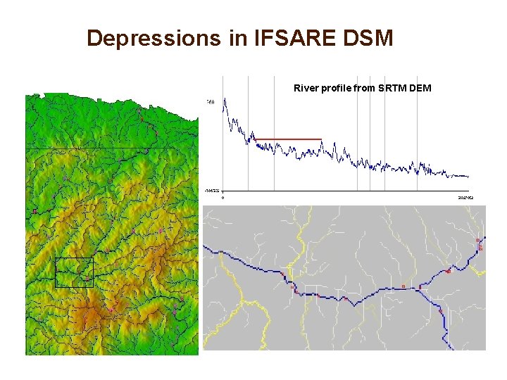
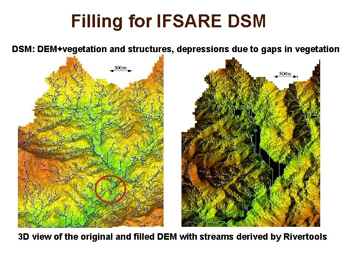
Depressions in IFSARE DSM River profile from SRTM DEM

Filling for IFSARE DSM: DEM+vegetation and structures, depressions due to gaps in vegetation 3 D view of the original and filled DEM with streams derived by Rivertools

Resolving large depression in IFSARE DSM most common approach: fill-in least cost path Both are SFD, D 8, 10 m resolution DEM

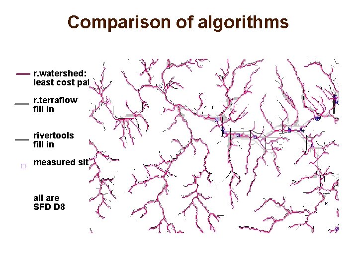
Comparison of algorithms r. watershed: least cost path r. terraflow fill in rivertools fill in measured sites all are SFD D 8

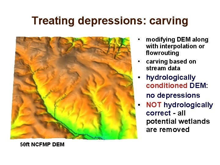
Treating depressions: carving • modifying DEM along with interpolation or flowrouting • carving based on stream data • hydrologically conditioned DEM: no depressions • NOT hydrologically correct - all potential wetlands are removed 50 ft NCFMP DEM

Stream extraction: accuracy Measured as horizontal accuracy of stream centerline or stream banks for large rivers • topographic maps - the lowest accuracy, old • extracted from lidar-based DEMs - better, but accuracy low in coastal plane, improvements expected with new lidar mapping • digitized from high res orthophotos and on ground surveys - most accurate except forested areas • structures require additional information (bridges are represented as dams in DEMs)

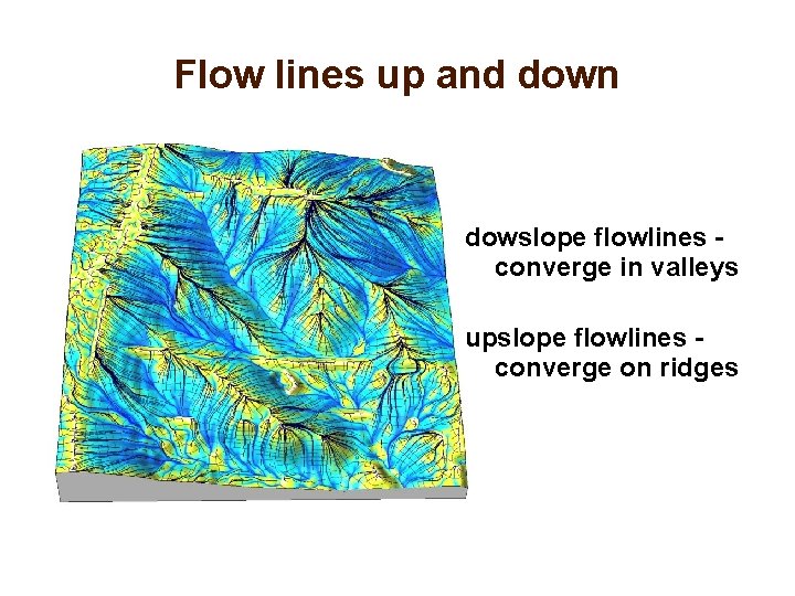
Flow lines up and down dowslope flowlines converge in valleys upslope flowlines converge on ridges

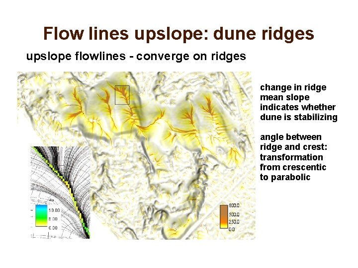
Flow lines upslope: dune ridges upslope flowlines - converge on ridges change in ridge mean slope indicates whether dune is stabilizing angle between ridge and crest: transformation from crescentic to parabolic

Watersheds • watershed - important land management unit • water and mass from a watershed drains to a single point: outlet • other terms for watershed: (drainage) basin, catchment, contributing area • watersheds can be organized into hierarchies based on the size of contributing area USGS Hydrologic units: drainage areas of major rivers or multiple smaller rivers: see more at http: //water. usgs. gov/GIS/huc. html

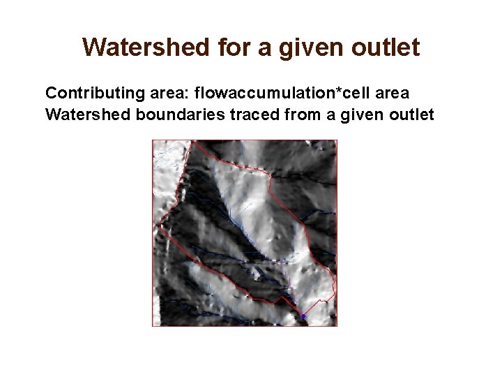
Watershed boundaries GIS watershed analysis: • find watershed boundaries for a given outlet contributing area from which water flows into a given grid cell or stream segment • partition area into watersheds with the given approximate size

Watershed boundaries • methods: same as for flow accumulation • starting from outlet, trace all cells going upslope using reversed flow direction and classify them with ID • snapping outlet to the stream - why it is needed • incomplete contributing area - given DEM does not cover entire drainage basin - flow accumulation and contributing area cannot be computed (handled e. g. , as negative values of flow accumulation)

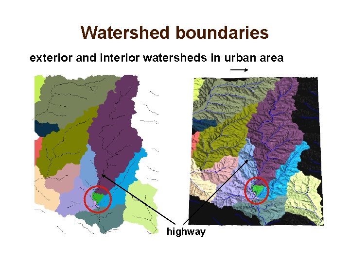
Watershed boundaries exterior and interior watersheds in urban area highway

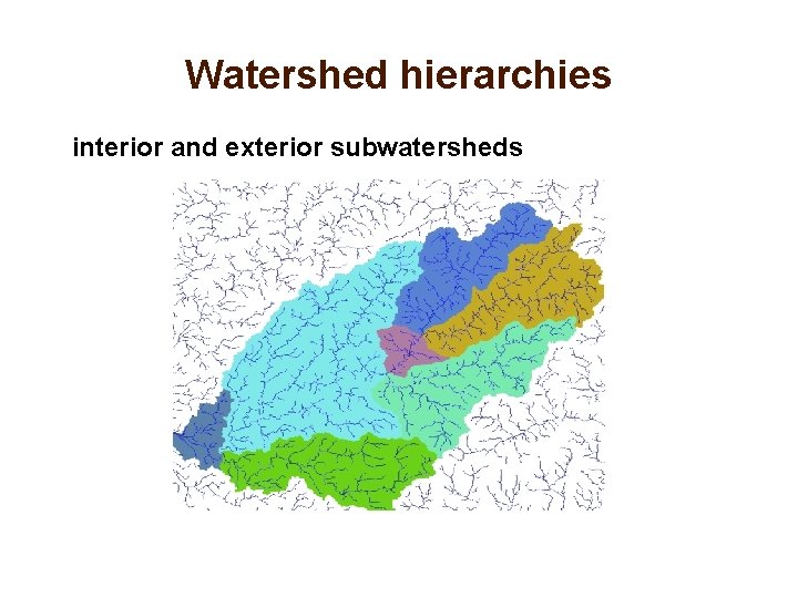
Watershed hierarchies interior and exterior subwatersheds

Watershed for a given outlet Contributing area: flowaccumulation*cell area Watershed boundaries traced from a given outlet

Watershed and stream data • EDNA - hydrologicaly relevant parameters from DEMs http: //edna. usgs. gov/ • Hydro. SHEDS worldwide watersheds and rivers based on 15 sec DEM derived from 90 m SRTM http: //hydrosheds. cr. usgs. gov/ • national hydrologic data set - USGS, from topomaps

Summary and references • Gruber and Peckham 2008, Chapter 7 in Hengl, T. and Reuter, H. I. , 2008, Geomorphometry: Concepts, Software, Applications, Elsevier • Chang Ch. 15, Neteler Ch. 5. 4. 4 • software: – – – JGRASS, Land. SERF Tau. DEM (Arc. GIS and Map. Window extension), TAS Terra. STREAM (for massive data sets), SAGA GIS, gv SIG