Final Exam Review Lecture 31 Administrivia Office hours

Final Exam Review Lecture 31

Administrivia • Office hours 1: 15 – 2: 15 today – also available via e-mail: ebenh@eecs. berkeley. edu – TAs will have extra office hours, • see class web page, news group • Final Exam May 16 8 -11 a. m. – Location: 55 Warren – Closed book, 2 pages of notes, both sides – IEEE will provide pastries and juice starting at 7: 30!

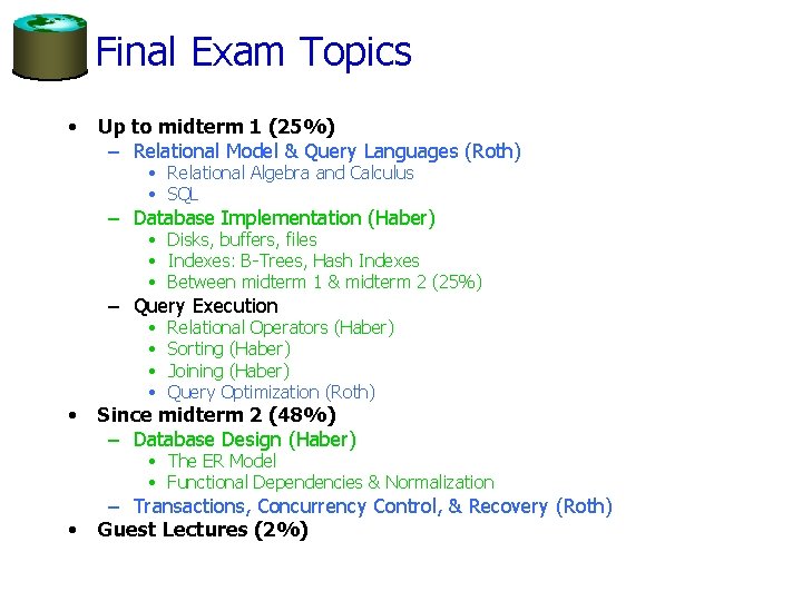
Final Exam Topics • Up to midterm 1 (25%) – Relational Model & Query Languages (Roth) • Relational Algebra and Calculus • SQL – Database Implementation (Haber) • Disks, buffers, files • Indexes: B-Trees, Hash Indexes • Between midterm 1 & midterm 2 (25%) – Query Execution • • • Relational Operators (Haber) Sorting (Haber) Joining (Haber) Query Optimization (Roth) Since midterm 2 (48%) – Database Design (Haber) • The ER Model • Functional Dependencies & Normalization • – Transactions, Concurrency Control, & Recovery (Roth) Guest Lectures (2%)

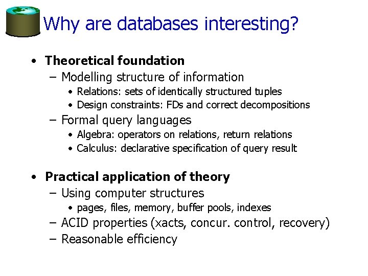
Why are databases interesting? • Theoretical foundation – Modelling structure of information • Relations: sets of identically structured tuples • Design constraints: FDs and correct decompositions – Formal query languages • Algebra: operators on relations, return relations • Calculus: declarative specification of query result • Practical application of theory – Using computer structures • pages, files, memory, buffer pools, indexes – ACID properties (xacts, concur. control, recovery) – Reasonable efficiency

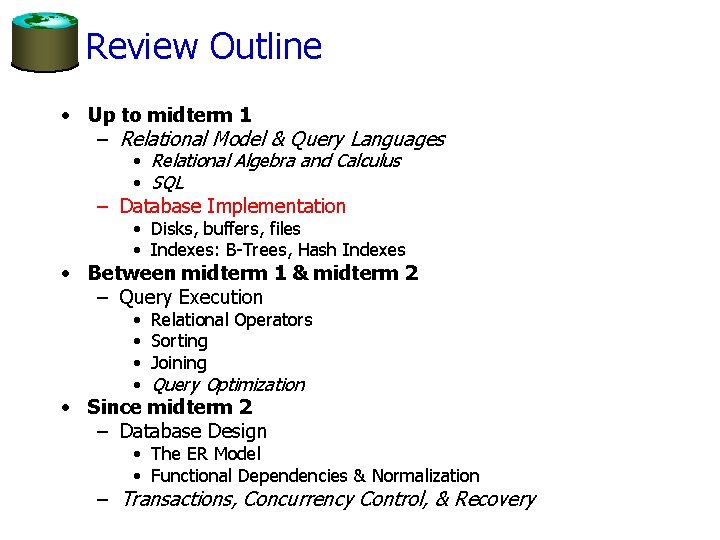
Review Outline • Up to midterm 1 – Relational Model & Query Languages • Relational Algebra and Calculus • SQL – Database Implementation • Disks, buffers, files • Indexes: B-Trees, Hash Indexes • Between midterm 1 & midterm 2 – Query Execution • • Relational Operators Sorting Joining Query Optimization • Since midterm 2 – Database Design • The ER Model • Functional Dependencies & Normalization – Transactions, Concurrency Control, & Recovery

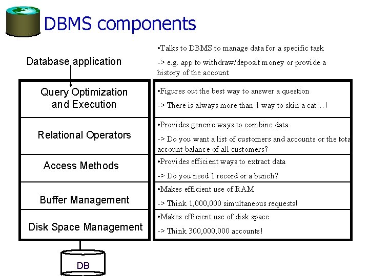
DBMS components • Talks to DBMS to manage data for a specific task Database application Query Optimization and Execution -> e. g. app to withdraw/deposit money or provide a history of the account • Figures out the best way to answer a question -> There is always more than 1 way to skin a cat…! • Provides generic ways to combine data Relational Operators Access Methods -> Do you want a list of customers and accounts or the total account balance of all customers? • Provides efficient ways to extract data -> Do you need 1 record or a bunch? • Makes efficient use of RAM Buffer Management -> Think 1, 000 simultaneous requests! • Makes efficient use of disk space Disk Space Management DB -> Think 300, 000 accounts!

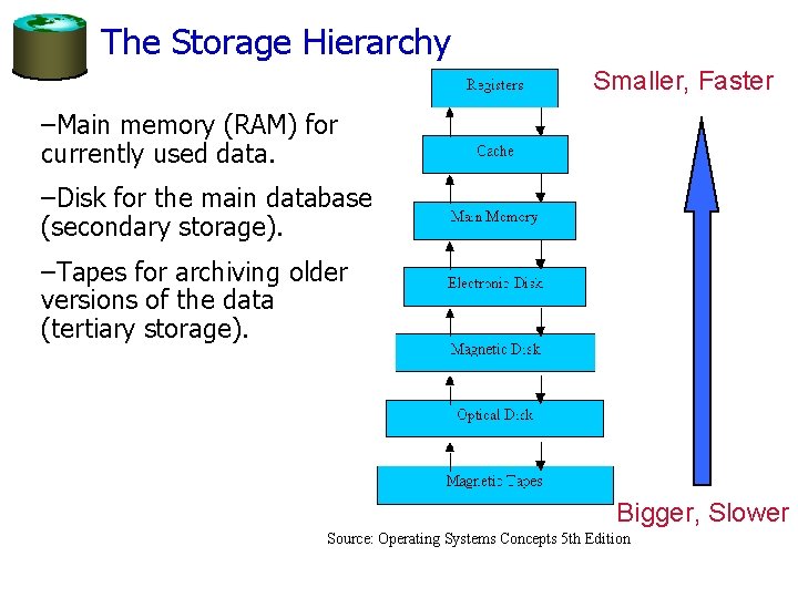
The Storage Hierarchy Smaller, Faster –Main memory (RAM) for currently used data. –Disk for the main database (secondary storage). –Tapes for archiving older versions of the data (tertiary storage). Bigger, Slower Source: Operating Systems Concepts 5 th Edition

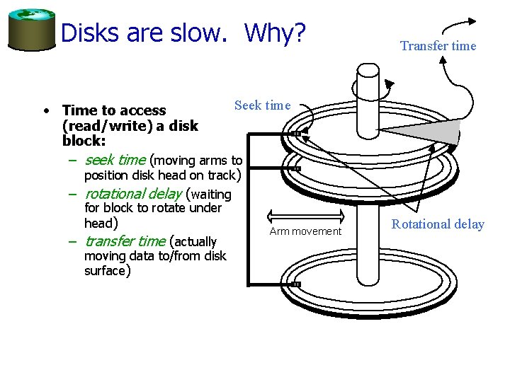
Disks are slow. Why? Transfer time Seek time • Time to access (read/write) a disk block: – seek time (moving arms to position disk head on track) – rotational delay (waiting for block to rotate under head) – transfer time (actually moving data to/from disk surface) Arm movement Rotational delay

Disk Space Manager • Lowest layer of DBMS software manages space on disk (using OS file system or not? ). • Higher levels call upon this layer to: – allocate/de-allocate a page – read/write a page • Best if a request for a sequence of pages is satisfied by pages stored sequentially on disk! – Responsibility of disk space manager. – Higher levels don’t know how this is done, or how free space is managed. – Though they make performance assumptions! • Hence disk space manager should do a decent job.

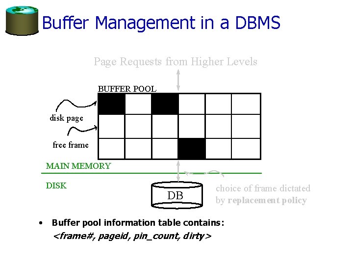
Buffer Management in a DBMS Page Requests from Higher Levels BUFFER POOL disk page free frame MAIN MEMORY DISK • DB choice of frame dictated by replacement policy Buffer pool information table contains: <frame#, pageid, pin_count, dirty>

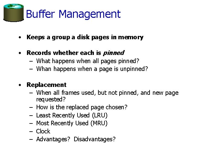
Buffer Management • Keeps a group a disk pages in memory • Records whether each is pinned – What happens when all pages pinned? – Whan happens when a page is unpinned? • Replacement – When all frames used, but not pinned, and new page requested? – How is the replaced page chosen? – Least Recently Used (LRU) – Most Recently Used (MRU) – Clock – Advantages? Disadvantages?

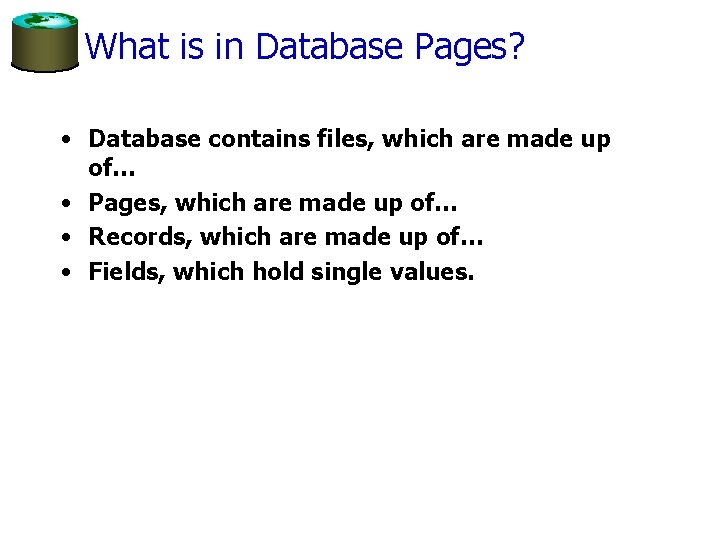
What is in Database Pages? • Database contains files, which are made up of… • Pages, which are made up of… • Records, which are made up of… • Fields, which hold single values.

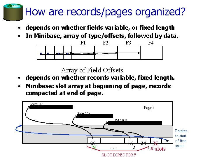
How are records/pages organized? • depends on whether fields variable, or fixed length • In Minibase, array of type/offsets, followed by data. F 1 F 2 F 3 F 4 Array of Field Offsets • depends on whether records variable, fixed length. • Minibase: slot array at beginning of page, records compacted at end of page. Rid = (i, N) Page i Rid = (i, 2) Rid = (i, 1) 20 N . . . 16 2 SLOT DIRECTORY 24 N 1 # slots Pointer to start of free space

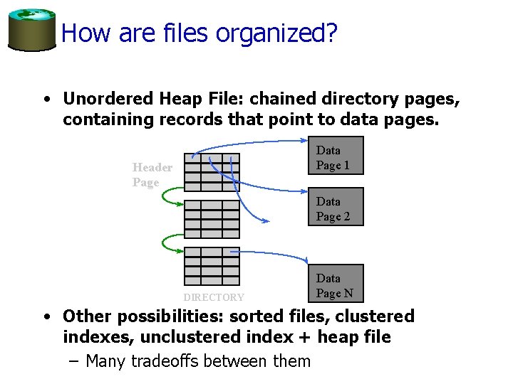
How are files organized? • Unordered Heap File: chained directory pages, containing records that point to data pages. Data Page 1 Header Page Data Page 2 DIRECTORY Data Page N • Other possibilities: sorted files, clustered indexes, unclustered index + heap file – Many tradeoffs between them

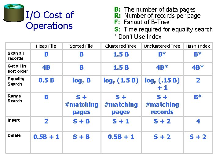
B: The number of data pages R: Number of records per page F: Fanout of B-Tree S: Time required for equality search * Don’t Use Index I/O Cost of Operations Heap File Sorted File Clustered Tree Unclustered Tree Hash Index B B 1. 5 B B* B* 4 B B 1. 5 B 4 B* Equality Search 0. 5 B log 2 B log. F (1. 5 B) log. F (. 15 B) +1 2 Range Search B S+ S+ #matching pages S+ #matching records B* Insert 2 S+B S+1 S+2 4 Delete 0. 5 B + 1 S+B 0. 5 B + 1 S+2 Scan all records Get all in sort order

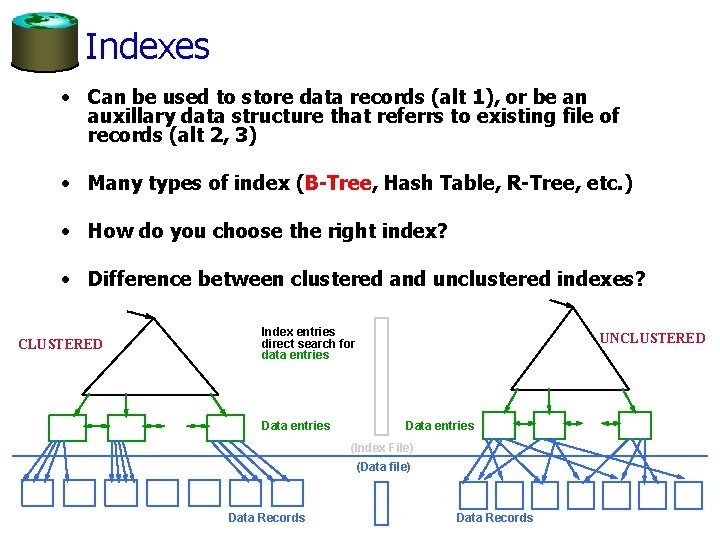
Indexes • Can be used to store data records (alt 1), or be an auxillary data structure that referrs to existing file of records (alt 2, 3) • Many types of index (B-Tree, Hash Table, R-Tree, etc. ) • How do you choose the right index? • Difference between clustered and unclustered indexes? CLUSTERED Index entries direct search for data entries Data entries UNCLUSTERED Data entries (Index File) (Data file) Data Records

Review Outline • Up to midterm 1 – Relational Model & Query Languages • Relational Algebra and Calculus • SQL – Database Implementation • Disks, buffers, files • Indexes: B-Trees, Hash Indexes • Between midterm 1 & midterm 2 – Query Execution • • Relational Operators Sorting Joining Query Optimization • Since midterm 2 – Database Design • The ER Model • Functional Dependencies & Normalization – Transactions, Concurrency Control, & Recovery

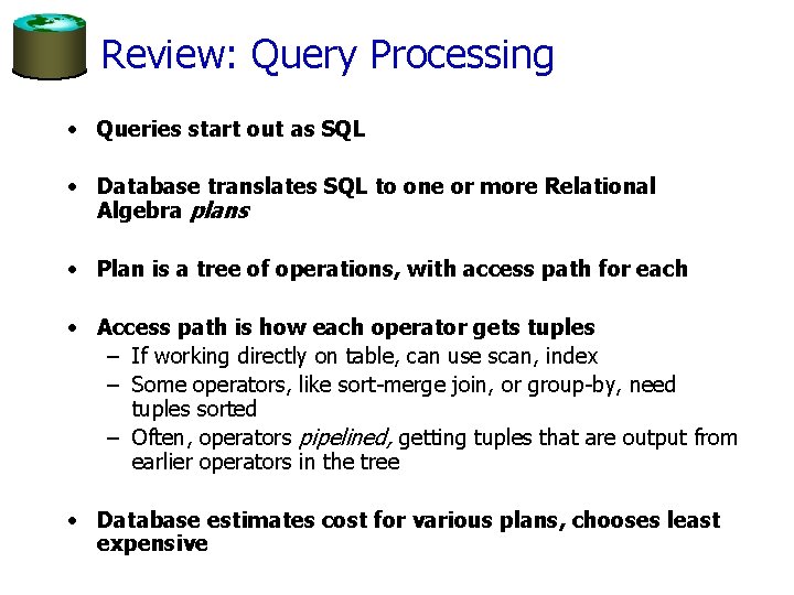
Review: Query Processing • Queries start out as SQL • Database translates SQL to one or more Relational Algebra plans • Plan is a tree of operations, with access path for each • Access path is how each operator gets tuples – If working directly on table, can use scan, index – Some operators, like sort-merge join, or group-by, need tuples sorted – Often, operators pipelined, getting tuples that are output from earlier operators in the tree • Database estimates cost for various plans, chooses least expensive

Cost of Operations • Selections • Projections • Sorting, a. k. a. Order By • Removing duplicates, a. k. a. Select Distinct • Joins

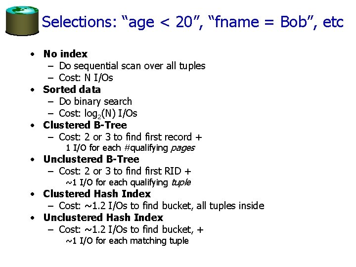
Selections: “age < 20”, “fname = Bob”, etc • No index – Do sequential scan over all tuples – Cost: N I/Os • Sorted data – Do binary search – Cost: log 2(N) I/Os • Clustered B-Tree – Cost: 2 or 3 to find first record + 1 I/O for each #qualifying pages • Unclustered B-Tree – Cost: 2 or 3 to find first RID + ~1 I/O for each qualifying tuple • Clustered Hash Index – Cost: ~1. 2 I/Os to find bucket, all tuples inside • Unclustered Hash Index – Cost: ~1. 2 I/Os to find bucket, + ~1 I/O for each matching tuple

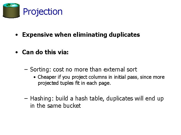
Projection • Expensive when eliminating duplicates • Can do this via: – Sorting: cost no more than external sort • Cheaper if you project columns in initial pass, since more projected tuples fit in each page. – Hashing: build a hash table, duplicates will end up in the same bucket

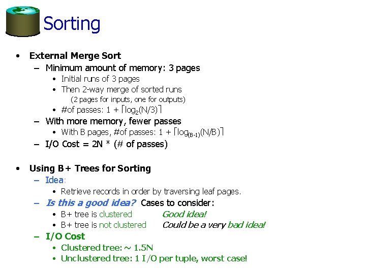
Sorting • External Merge Sort – Minimum amount of memory: 3 pages • Initial runs of 3 pages • Then 2 -way merge of sorted runs (2 pages for inputs, one for outputs) • #of passes: 1 + log 2(N/3) – With more memory, fewer passes • With B pages, #of passes: 1 + log(B-1)(N/B) – I/O Cost = 2 N * (# of passes) • Using B+ Trees for Sorting – Idea: • Retrieve records in order by traversing leaf pages. – Is this a good idea? Cases to consider: • B+ tree is clustered • B+ tree is not clustered Good idea! Could be a very bad idea! – I/O Cost • Clustered tree: ~ 1. 5 N • Unclustered tree: 1 I/O per tuple, worst case!

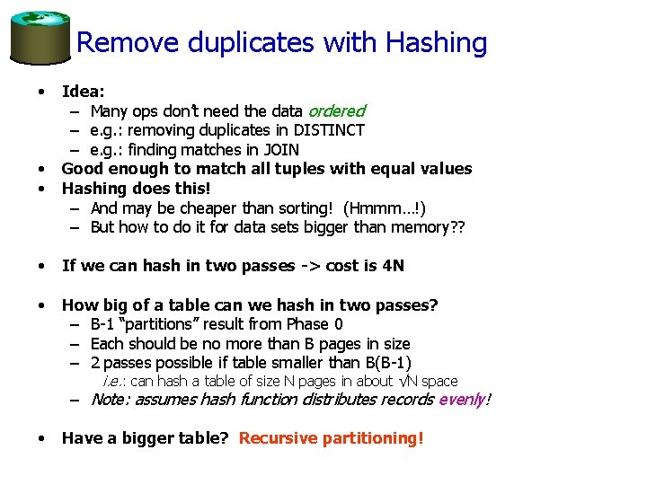
Remove duplicates with Hashing • • • Idea: – Many ops don’t need the data ordered – e. g. : removing duplicates in DISTINCT – e. g. : finding matches in JOIN Good enough to match all tuples with equal values Hashing does this! – And may be cheaper than sorting! (Hmmm…!) – But how to do it for data sets bigger than memory? ? • If we can hash in two passes -> cost is 4 N • How big of a table can we hash in two passes? – B-1 “partitions” result from Phase 0 – Each should be no more than B pages in size – 2 passes possible if table smaller than B(B-1) i. e. : can hash a table of size N pages in about √N space – Note: assumes hash function distributes records evenly! • Have a bigger table? Recursive partitioning!

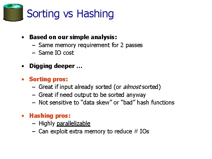
Sorting vs Hashing • Based on our simple analysis: – Same memory requirement for 2 passes – Same IO cost • Digging deeper … • Sorting pros: – Great if input already sorted (or almost sorted) – Great if need output to be sorted anyway – Not sensitive to “data skew” or “bad” hash functions • Hashing pros: – Highly parallelizable – Can exploit extra memory to reduce # IOs

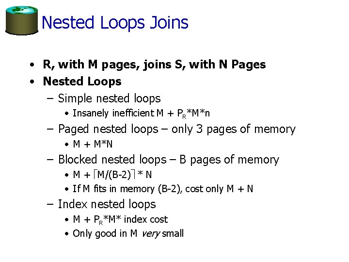
Nested Loops Joins • R, with M pages, joins S, with N Pages • Nested Loops – Simple nested loops • Insanely inefficient M + PR*M*n – Paged nested loops – only 3 pages of memory • M + M*N – Blocked nested loops – B pages of memory • M + M/(B-2) * N • If M fits in memory (B-2), cost only M + N – Index nested loops • M + PR*M* index cost • Only good in M very small

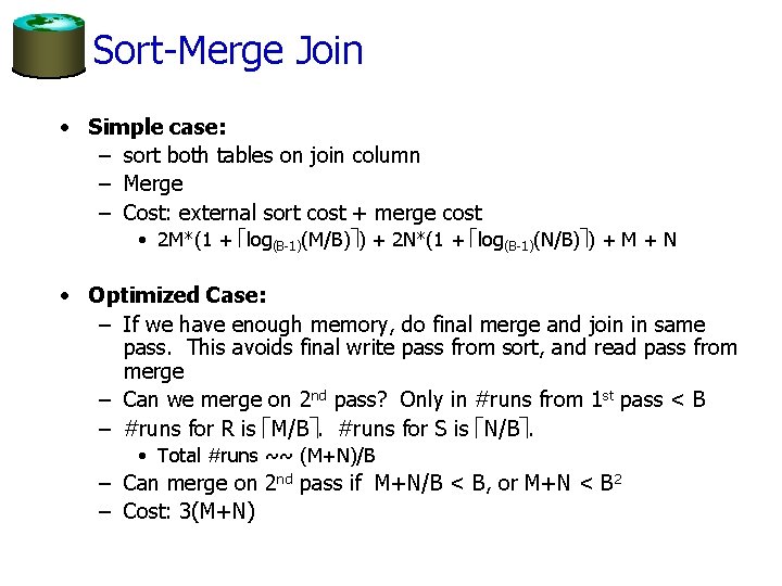
Sort-Merge Join • Simple case: – sort both tables on join column – Merge – Cost: external sort cost + merge cost • 2 M*(1 + log(B-1)(M/B) ) + 2 N*(1 + log(B-1)(N/B) ) + M + N • Optimized Case: – If we have enough memory, do final merge and join in same pass. This avoids final write pass from sort, and read pass from merge – Can we merge on 2 nd pass? Only in #runs from 1 st pass < B – #runs for R is M/B. #runs for S is N/B. • Total #runs ~~ (M+N)/B – Can merge on 2 nd pass if M+N/B < B, or M+N < B 2 – Cost: 3(M+N)

Cost of Hash Join • Partitioning phase: read+write both relations 2(|R|+|S|) I/Os • Matching phase: read+write both relations |R|+|S| I/Os • Total cost of 2 -pass hash join = 3(|R|+|S|) Q: what is cost of 2 -pass merge-sort join? Q: how much memory needed for 2 -pass hash join?

Summary: Hashing vs. Sorting • Sorting pros: – Good if input already sorted, or need output sorted – Not sensitive to data skew or bad hash functions • Hashing pros: – Often cheaper due to hybrid hashing – For join: # passes depends on size of smaller relation – Highly parallelizable

Review Outline • Up to midterm 1 – Relational Model & Query Languages • Relational Algebra and Calculus • SQL – Database Implementation • Disks, buffers, files • Indexes: B-Trees, Hash Indexes • Between midterm 1 & midterm 2 – Query Execution • • Relational Operators Sorting Joining Query Optimization • Since midterm 2 – Database Design • The ER Model • Functional Dependencies & Normalization – Transactions, Concurrency Control, & Recovery

Review: Database Design • Requirements Analysis – user needs; what must database do? • Conceptual Design – high level descr (often done w/ER model) • Logical Design – translate ER into DBMS data model • Schema Refinement – consistency, normalization • Physical Design - indexes, disk layout • Security Design - who accesses what

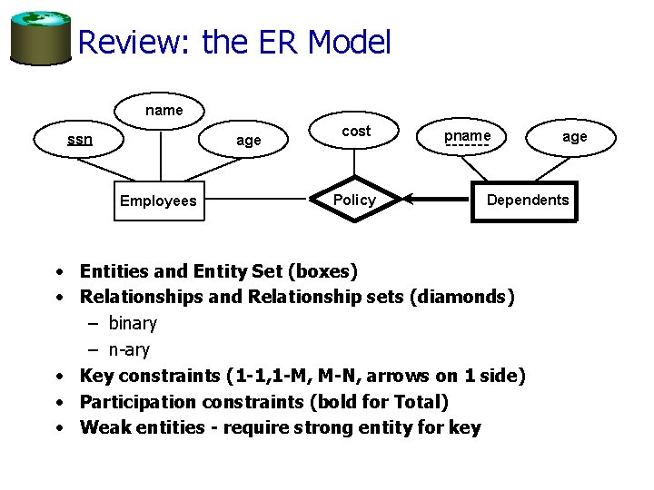
Review: the ER Model name ssn age Employees cost Policy pname age Dependents • Entities and Entity Set (boxes) • Relationships and Relationship sets (diamonds) – binary – n-ary • Key constraints (1 -1, 1 -M, M-N, arrows on 1 side) • Participation constraints (bold for Total) • Weak entities - require strong entity for key

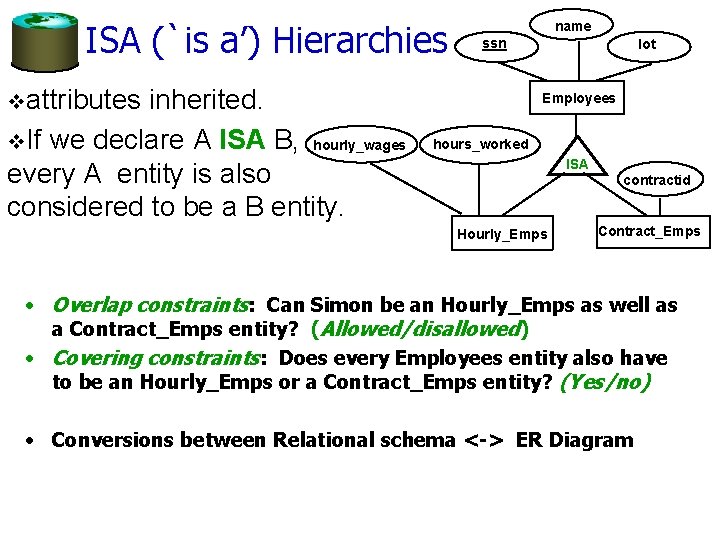
ISA (`is a’) Hierarchies inherited. v. If we declare A ISA B, hourly_wages every A entity is also considered to be a B entity. name ssn vattributes lot Employees hours_worked ISA Hourly_Emps contractid Contract_Emps • Overlap constraints: Can Simon be an Hourly_Emps as well as a Contract_Emps entity? (Allowed/disallowed) • Covering constraints: Does every Employees entity also have to be an Hourly_Emps or a Contract_Emps entity? (Yes/no) • Conversions between Relational schema <-> ER Diagram

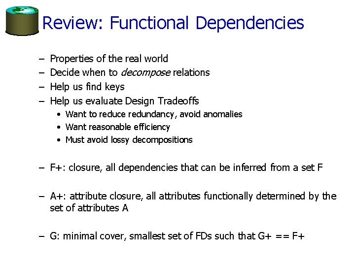
Review: Functional Dependencies – – Properties of the real world Decide when to decompose relations Help us find keys Help us evaluate Design Tradeoffs • Want to reduce redundancy, avoid anomalies • Want reasonable efficiency • Must avoid lossy decompositions – F+: closure, all dependencies that can be inferred from a set F – A+: attribute closure, all attributes functionally determined by the set of attributes A – G: minimal cover, smallest set of FDs such that G+ == F+

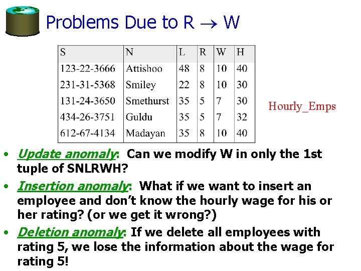
Problems Due to R W Hourly_Emps • Update anomaly: Can we modify W in only the 1 st tuple of SNLRWH? • Insertion anomaly: What if we want to insert an employee and don’t know the hourly wage for his or her rating? (or we get it wrong? ) • Deletion anomaly: If we delete all employees with rating 5, we lose the information about the wage for rating 5!

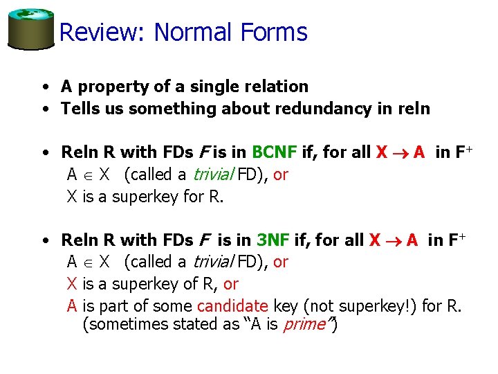
Review: Normal Forms • A property of a single relation • Tells us something about redundancy in reln • Reln R with FDs F is in BCNF if, for all X A in F+ A X (called a trivial FD), or X is a superkey for R. • Reln R with FDs F is in 3 NF if, for all X A in F+ A X (called a trivial FD), or X is a superkey of R, or A is part of some candidate key (not superkey!) for R. (sometimes stated as “A is prime”)

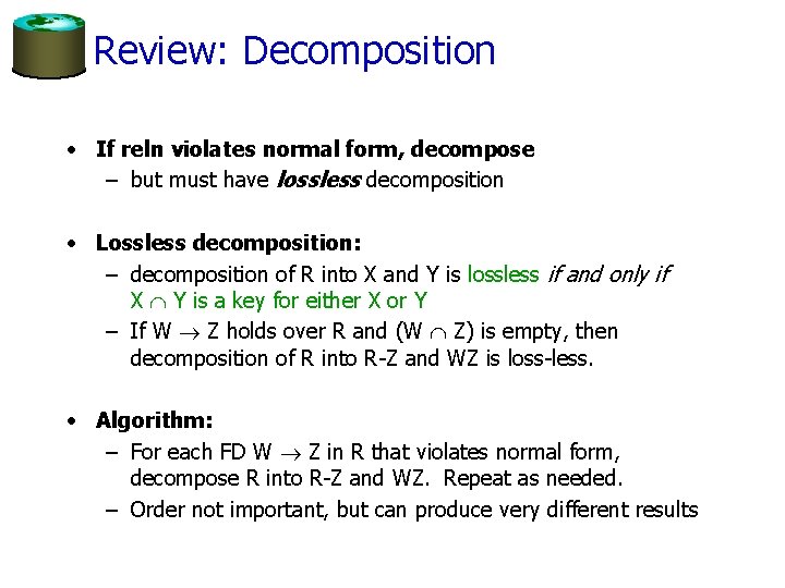
Review: Decomposition • If reln violates normal form, decompose – but must have lossless decomposition • Lossless decomposition: – decomposition of R into X and Y is lossless if and only if X Y is a key for either X or Y – If W Z holds over R and (W Z) is empty, then decomposition of R into R-Z and WZ is loss-less. • Algorithm: – For each FD W Z in R that violates normal form, decompose R into R-Z and WZ. Repeat as needed. – Order not important, but can produce very different results

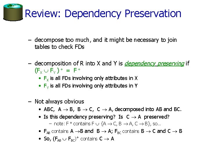
Review: Dependency Preservation – decompose too much, and it might be necessary to join tables to check FDs – decomposition of R into X and Y is dependency preserving if (FX FY ) + = F + • FX is all FDs involving only attributes in X • FY is all FDs involving only attributes in Y – Not always obvious • ABC, A B, B C, C A, decomposed into AB and BC. • Is this dependency preserving? Is C A preserved? – note: F + contains F {A C, B A, C B}, so… • FAB contains A B and B A; FBC contains B C and C B • So, (FAB FBC)+ contains C A

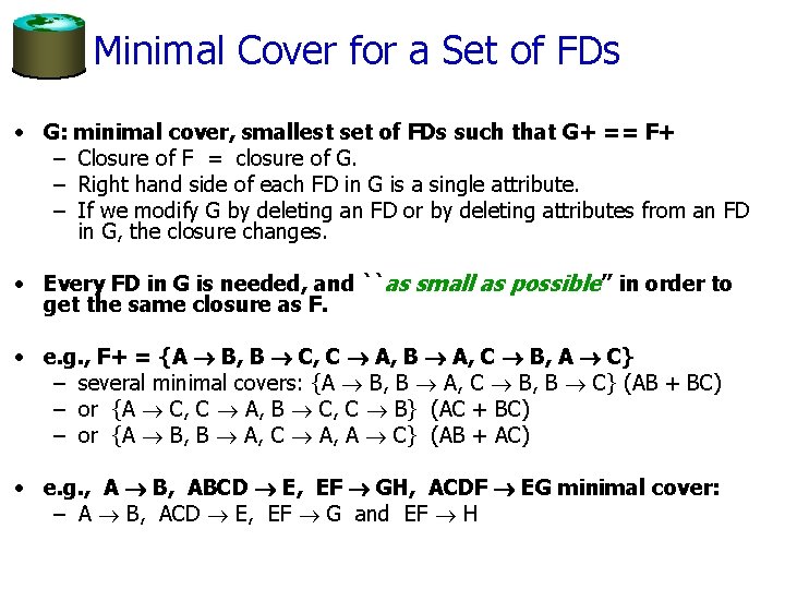
Minimal Cover for a Set of FDs • G: minimal cover, smallest set of FDs such that G+ == F+ – Closure of F = closure of G. – Right hand side of each FD in G is a single attribute. – If we modify G by deleting an FD or by deleting attributes from an FD in G, the closure changes. • Every FD in G is needed, and ``as small as possible’’ in order to get the same closure as F. • e. g. , F+ = {A B, B C, C A, B A, C B, A C} – several minimal covers: {A B, B A, C B, B C} (AB + BC) – or {A C, C A, B C, C B} (AC + BC) – or {A B, B A, C A, A C} (AB + AC) • e. g. , A B, ABCD E, EF GH, ACDF EG minimal cover: – A B, ACD E, EF G and EF H

BCNF and Dependency Preservation • In general, there may not be a dependency preserving decomposition into BCNF. • But, you can always find dependency-preserving decomposition into 3 NF – Top down: • Decompose until it is in 3 NF • Compute minimal cover for FDs • If minimal cover contains a FD X Y is not preserved, add reln XY – Bottom up: • Compute minimal cover • For each FD X Y in minimal cover, create reln XY – Why does this work? Minimal cover doesn’t include redundant transitive dependencies, which don’t need to be preserved

Questions? • Up to midterm 1 – Relational Model & Query Languages • Relational Algebra and Calculus • SQL – Database Implementation • Disks, buffers, files • Indexes: B-Trees, Hash Indexes • Between midterm 1 & midterm 2 – Query Execution • • Relational Operators Sorting Joining Query Optimization • Since midterm 2 – Database Design • The ER Model • Functional Dependencies & Normalization – Transactions, Concurrency Control, & Recovery

Thank you! • See you next Wednesday.