Extrapolation Models for Convergence Acceleration and Functions Extension

Extrapolation Models for Convergence Acceleration and Function’s Extension David Levin Tel-Aviv University MAIA Erice 2013

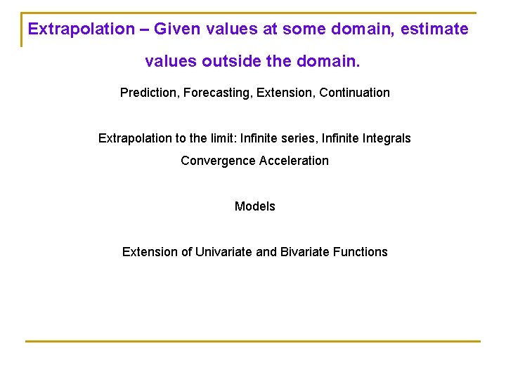
Extrapolation – Given values at some domain, estimate values outside the domain. Prediction, Forecasting, Extension, Continuation Extrapolation to the limit: Infinite series, Infinite Integrals Convergence Acceleration Models Extension of Univariate and Bivariate Functions

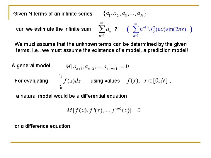
Given N terms of an infinite series can we estimate the infinite sum ? We must assume that the unknown terms can be determined by the given terms, i. e. , we must assume the existence of a model, a prediction model! A general model: For evaluating using values a natural model would be a differential equation or a difference equation. ,

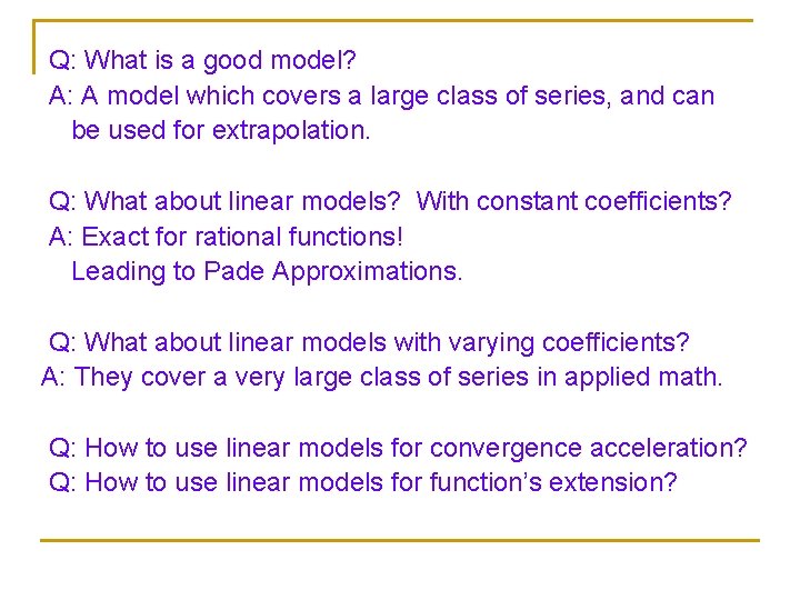
Q: What is a good model? A: A model which covers a large class of series, and can be used for extrapolation. Q: What about linear models? With constant coefficients? A: Exact for rational functions! Leading to Pade Approximations. Q: What about linear models with varying coefficients? A: They cover a very large class of series in applied math. Q: How to use linear models for convergence acceleration? Q: How to use linear models for function’s extension?

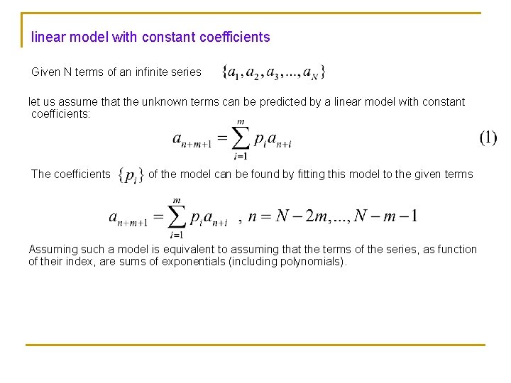
linear model with constant coefficients Given N terms of an infinite series let us assume that the unknown terms can be predicted by a linear model with constant coefficients: The coefficients of the model can be found by fitting this model to the given terms Assuming such a model is equivalent to assuming that the terms of the series, as function of their index, are sums of exponentials (including polynomials).

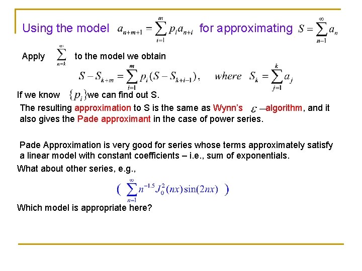
Using the model Apply for approximating to the model we obtain If we know we can find out S. The resulting approximation to S is the same as Wynn’s algorithm, and it also gives the Pade approximant in the case of power series. Pade Approximation is very good for series whose terms approximately satisfy a linear model with constant coefficients – i. e. , sum of exponentials. What about other series, e. g. , Which model is appropriate here?

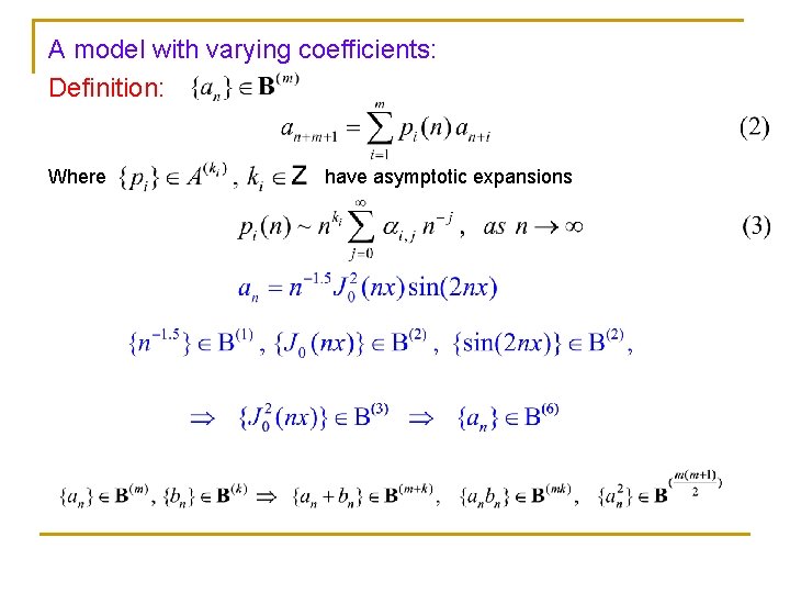
A model with varying coefficients: Definition: Where have asymptotic expansions

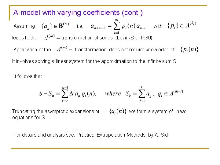
A model with varying coefficients (cont. ) Assuming leads to the Application of the , i. e. , with transformation of series (Levin-Sidi 1980). transformation does not require knowledge of It involves solving a linear system for the approximation to the infinite sum S. It follows that Truncating the asymptotic expansions of equations for S. we form a system of linear For details and analysis see: Practical Extrapolation Methods, by A. Sidi

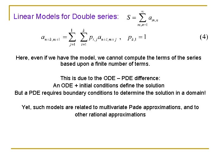
Linear Models for Double series: Here, even if we have the model, we cannot compute the terms of the series based upon a finite number of terms. This is due to the ODE – PDE difference: An ODE + initial conditions define the solution But a PDE requires boundary conditions to determine the solution in a domain! Yet, such models are related to multivariate Pade approximations, and to other rational approximations

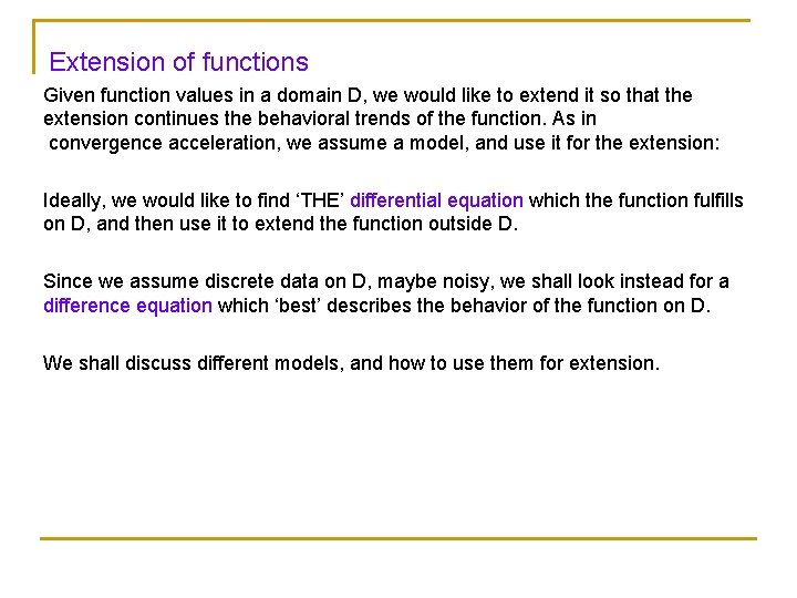
Extension of functions Given function values in a domain D, we would like to extend it so that the extension continues the behavioral trends of the function. As in convergence acceleration, we assume a model, and use it for the extension: Ideally, we would like to find ‘THE’ differential equation which the function fulfills on D, and then use it to extend the function outside D. Since we assume discrete data on D, maybe noisy, we shall look instead for a difference equation which ‘best’ describes the behavior of the function on D. We shall discuss different models, and how to use them for extension.

Linear Model – Constant Coef. – Univariate case Given function values in [a, b]: Assume f is bandlimited, and let By Nyquist–Shannon sampling theorem sampling distance d is sufficient for reconstructing f. We use sequences of ‘mesh size’ To these sequences we fit a Linear Constant Coefficients Model of order m using least-squares minimization to find the model coefficients:

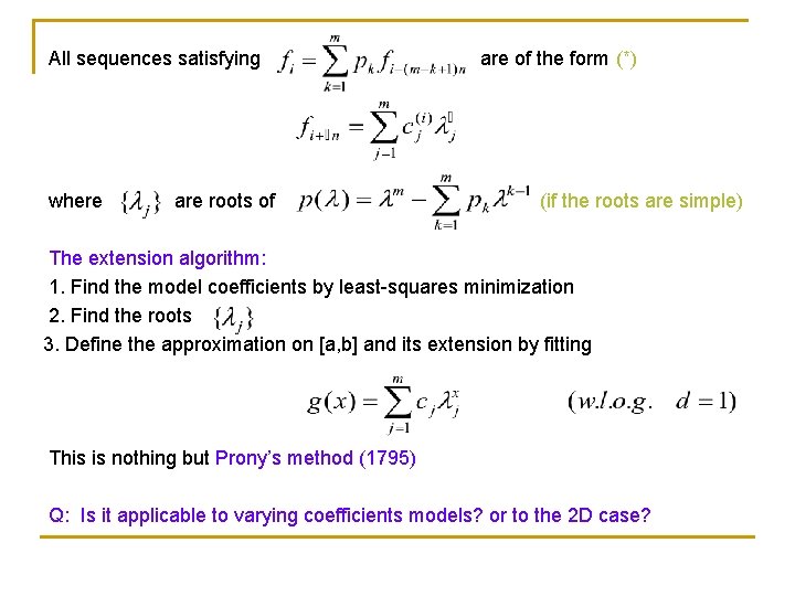
All sequences satisfying where are roots of are of the form (*) (if the roots are simple) The extension algorithm: 1. Find the model coefficients by least-squares minimization 2. Find the roots 3. Define the approximation on [a, b] and its extension by fitting This is nothing but Prony’s method (1795) Q: Is it applicable to varying coefficients models? or to the 2 D case?

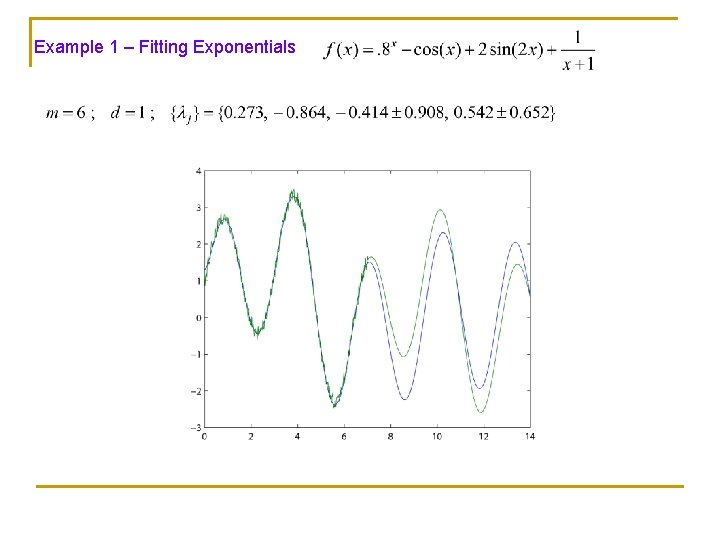
Example 1 – Fitting Exponentials

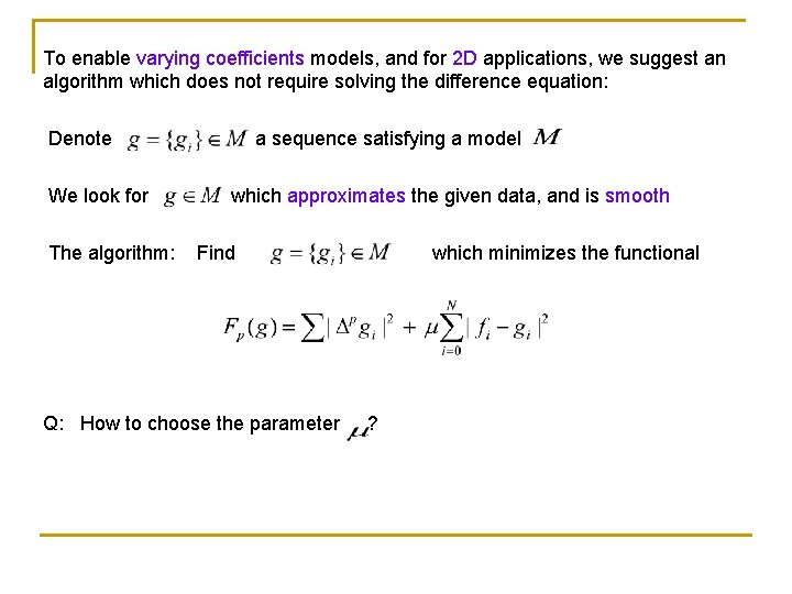
To enable varying coefficients models, and for 2 D applications, we suggest an algorithm which does not require solving the difference equation: Denote We look for The algorithm: a sequence satisfying a model which approximates the given data, and is smooth Find Q: How to choose the parameter which minimizes the functional ?

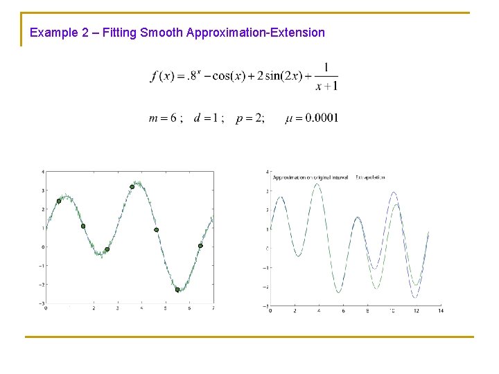
Example 2 – Fitting Smooth Approximation-Extension

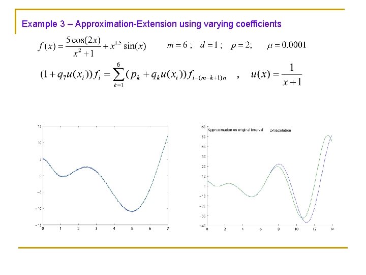
Example 3 – Approximation-Extension using varying coefficients

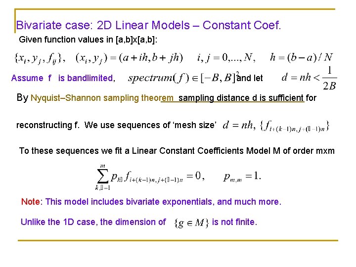
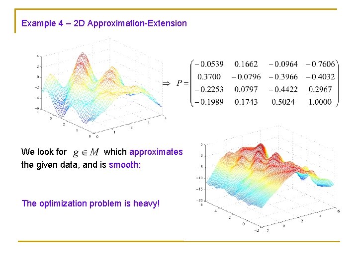
Bivariate case: 2 D Linear Models – Constant Coef. Given function values in [a, b]x[a, b]: Assume f is bandlimited, and let By Nyquist–Shannon sampling theorem sampling distance d is sufficient for reconstructing f. We use sequences of ‘mesh size’ To these sequences we fit a Linear Constant Coefficients Model M of order mxm Note: This model includes bivariate exponentials, and much more. Unlike the 1 D case, the dimension of is not finite.

Example 4 – 2 D Approximation-Extension We look for which approximates the given data, and is smooth: The optimization problem is heavy!

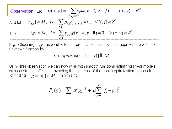
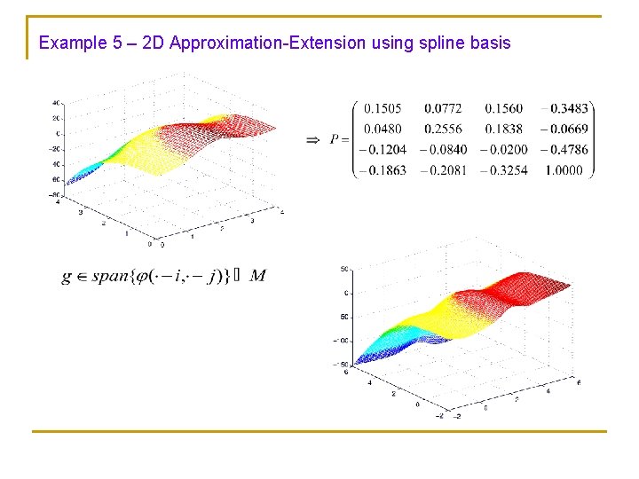
Observation: Let And let then ----------------------------------------------------------E. g. , Choosing as a cubic tensor product B-spline, we can approximate well the unknown function by Using this observation we can now work with smooth functions satisfying linear models with constant coefficients, avoiding the high cost of the above optimization approach of finding minimizing

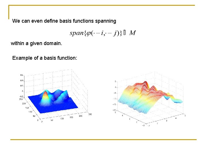
We can even define basis functions spanning within a given domain. Example of a basis function:

Example 5 – 2 D Approximation-Extension using spline basis

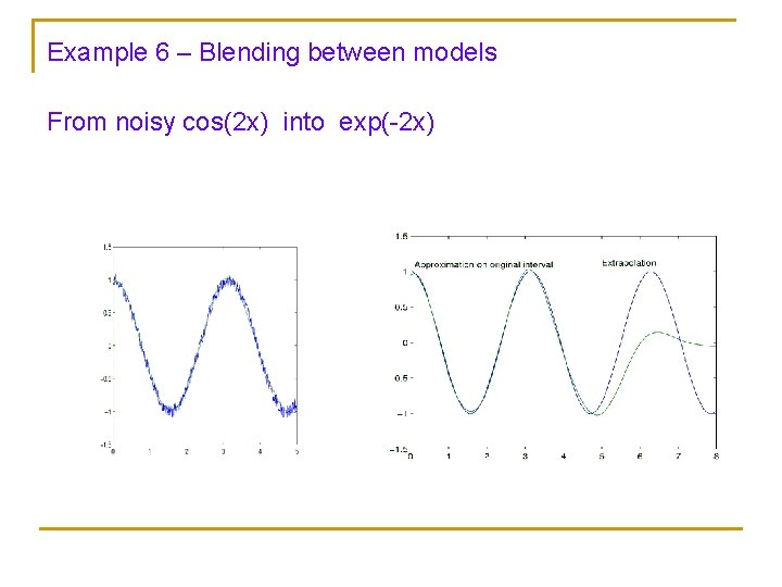
Example 6 – Blending between models From noisy cos(2 x) into exp(-2 x)

Thank you!