Introduction Convergence Convergence Convergence Convergence If u and






- Slides: 58

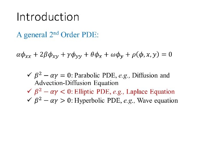
Introduction •

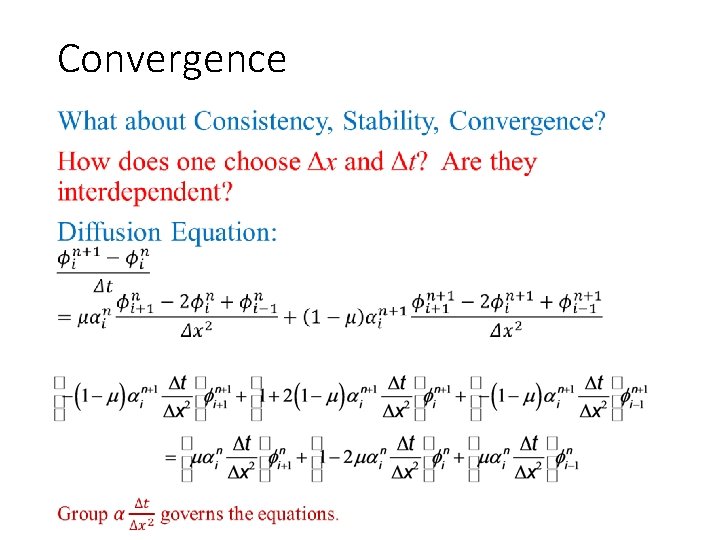
Convergence •

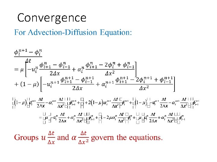
Convergence •

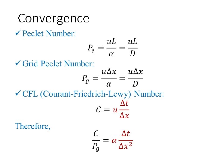
Convergence •

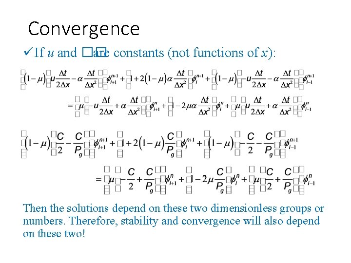
Convergence ü If u and �� are constants (not functions of x): Then the solutions depend on these two dimensionless groups or numbers. Therefore, stability and convergence will also depend on these two!

Consistency •

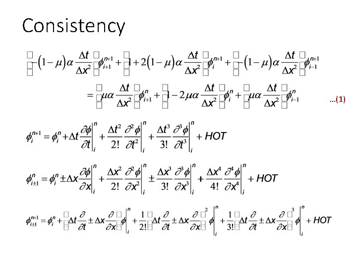
Consistency …(1)

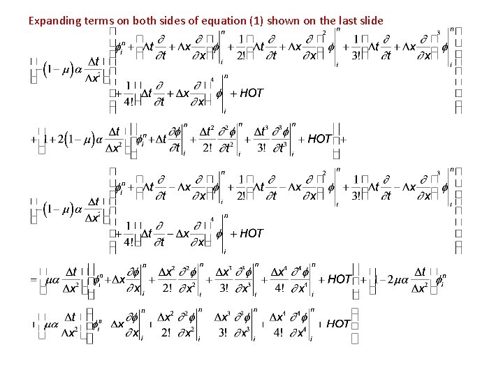
Expanding terms on both sides of equation (1) shown on the last slide

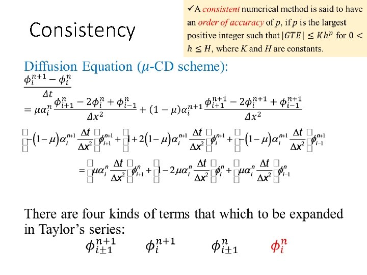
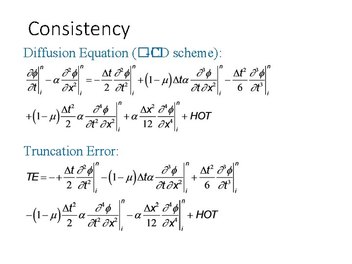
Consistency Diffusion Equation (�� -CD scheme): Truncation Error:

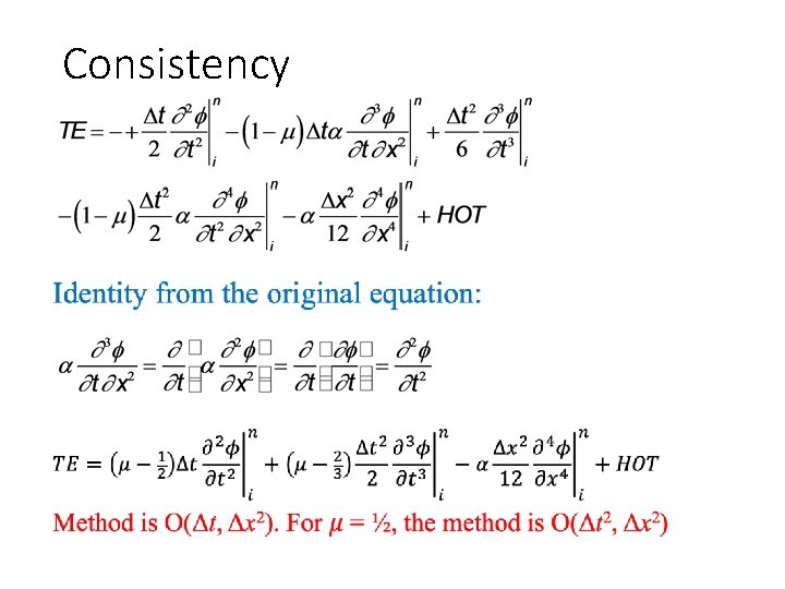
Consistency •

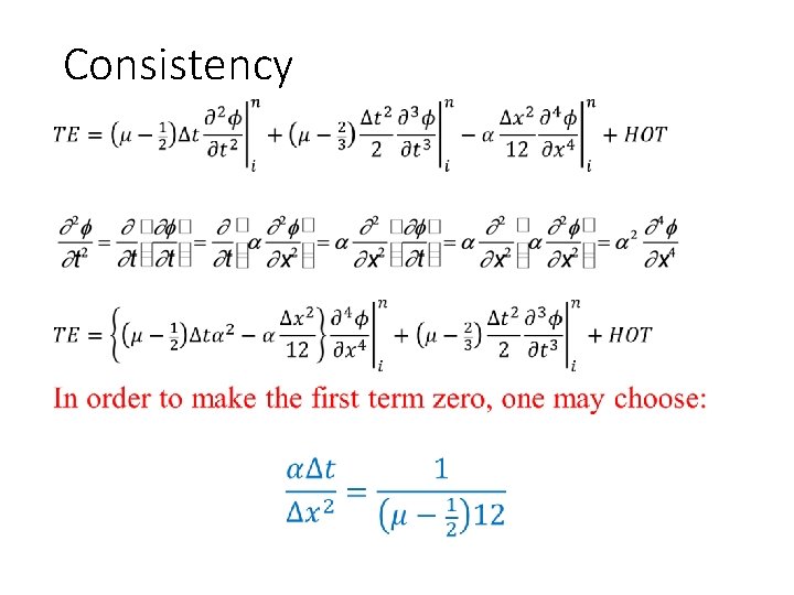
Consistency •

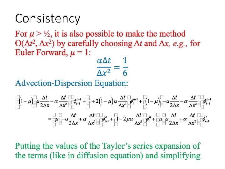
Consistency •

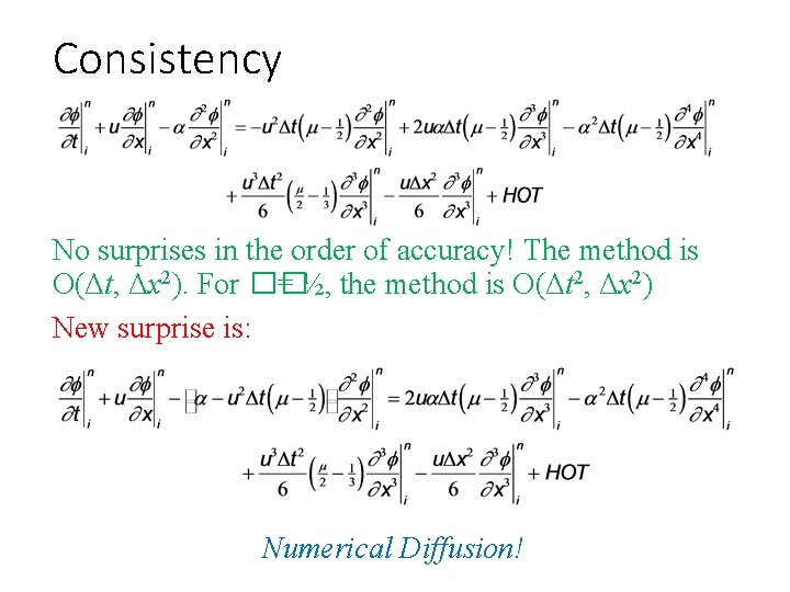
Consistency No surprises in the order of accuracy! The method is O(Δt, Δx 2). For �� = ½, the method is O(Δt 2, Δx 2) New surprise is: Numerical Diffusion!

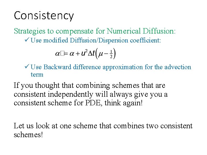
Consistency Strategies to compensate for Numerical Diffusion: ü Use modified Diffusion/Dispersion coefficient: ü Use Backward difference approximation for the advection term If you thought that combining schemes that are consistent independently will always give you a consistent scheme for PDE, think again! Let us look at one scheme that combines two consistent schemes!

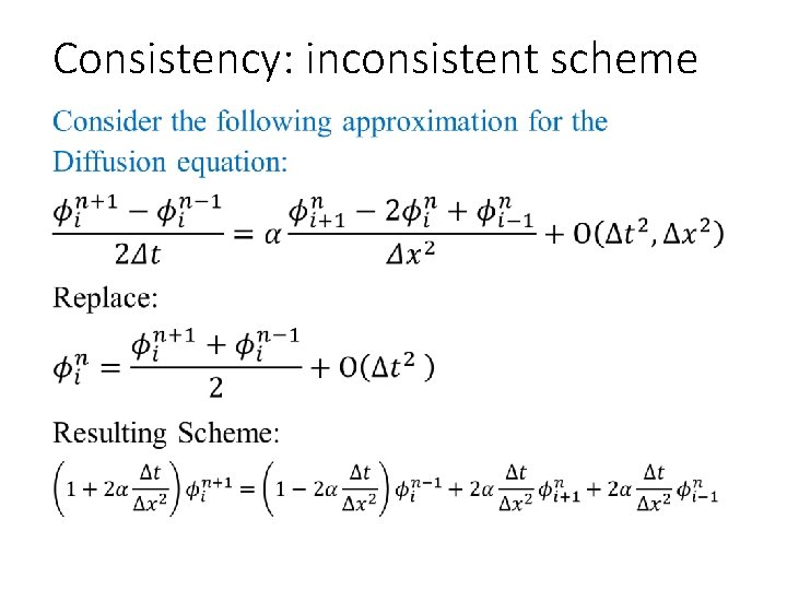
Consistency: inconsistent scheme •

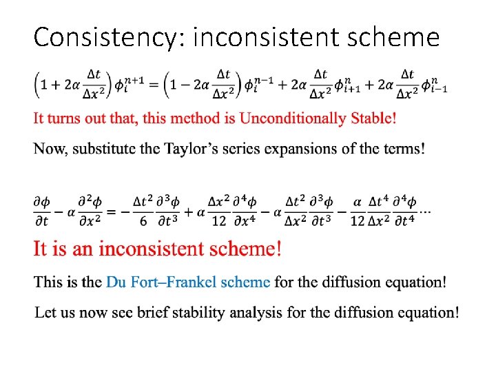
Consistency: inconsistent scheme •

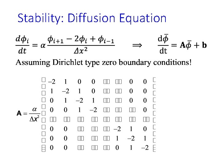
Stability: Diffusion Equation •

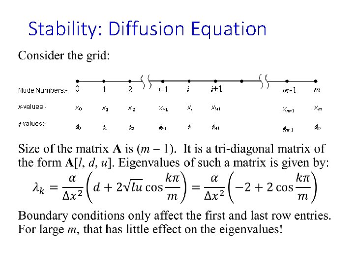
Stability: Diffusion Equation •

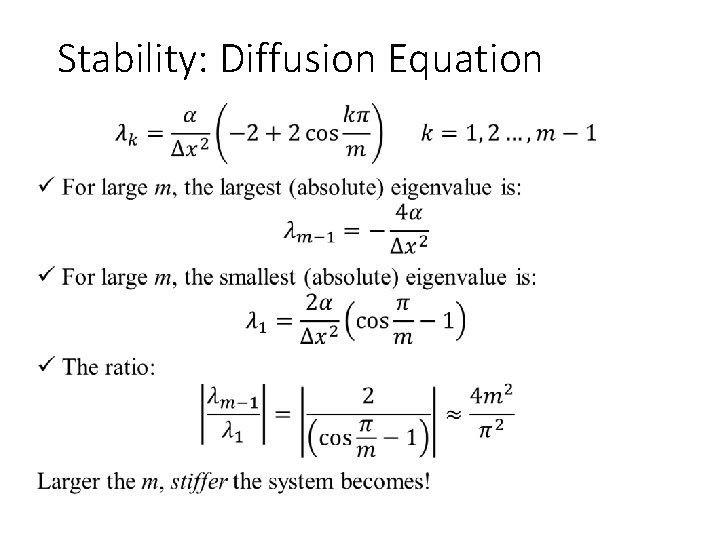
Stability: Diffusion Equation •

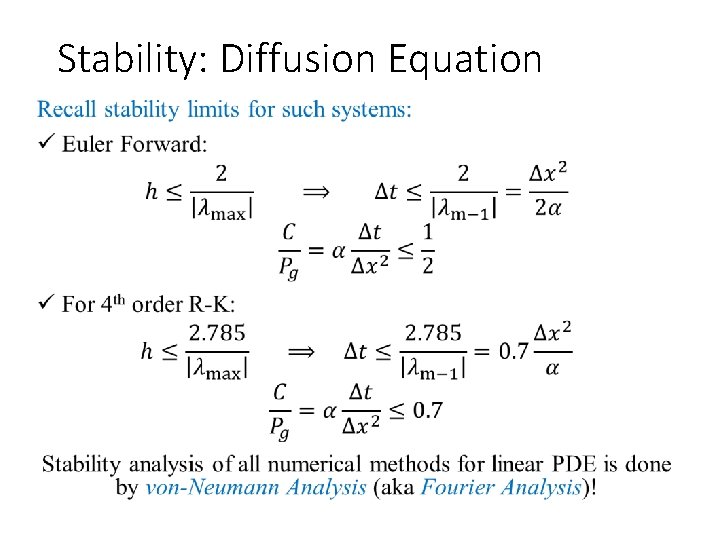
Stability: Diffusion Equation •

ESO 208 A: Computational Methods in Engineering Partial Differential Equation: Elliptic Equation Department of Civil Engineering IIT Kanpur

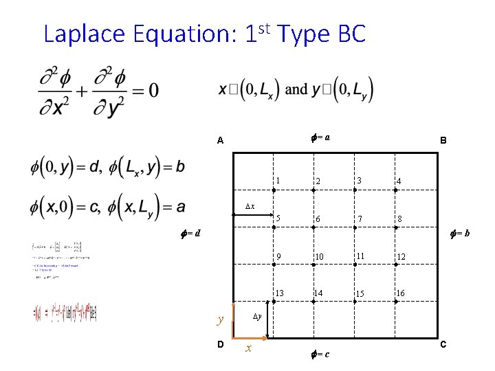
Laplace Equation: 1 st Type BC f=a A B 1 2 3 4 5 6 7 8 Dx f=d f=b 10 11 12 13 14 15 16 Dy y D 9 x f=c C

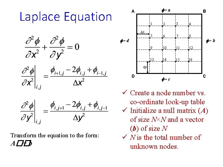
Laplace Equation f=a A Dx f=d B 1 2 3 4 5 6 7 8 9 10 11 12 13 14 15 16 f=b Dy D Transform the equation to the form: A�� =b f=c C ü Create a node number vs. co-ordinate look-up table ü Initialize a null matrix (A) of size N×N and a vector (b) of size N ü N is the total number of unknown nodes.

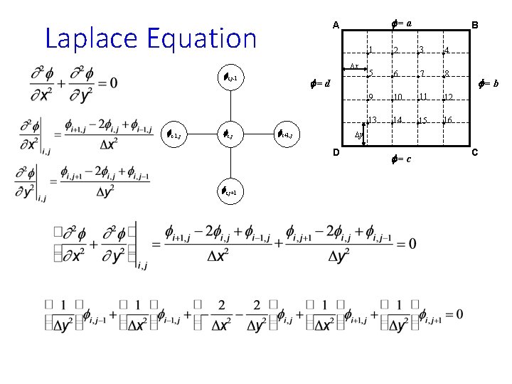
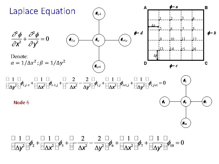
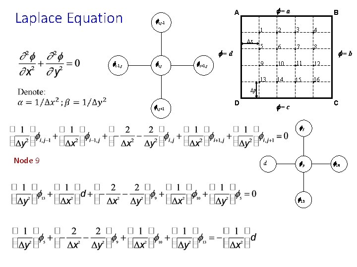
Laplace Equation Dx fi, j-1 fi-1, j fi, j f=d fi+1, j B 1 2 3 4 5 6 7 8 9 10 11 12 13 14 15 16 f=b Dy D fi, j+1 f=a A f=c C

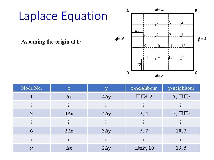
Laplace Equation f=a A Dx f=d Assuming the origin at D B 1 2 3 4 5 6 7 8 9 10 11 12 13 14 15 16 f=b Dy D C f=c Node No. x y x-neighbour y-neighbour 1 Δx 4Δy �� = d, 2 5, �� =a 3 3Δx 4Δy 2, 4 7, �� =a 6 2Δx 3Δy 5, 7 10, 2 9 Δx 2Δy �� = d, 10 13, 5

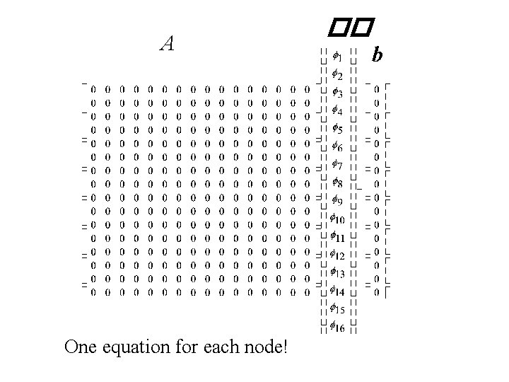
A One equation for each node! �� b

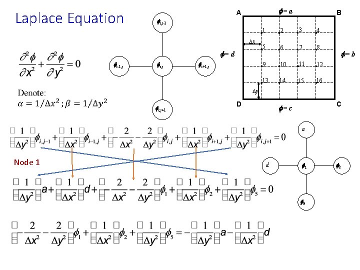
Laplace Equation f=a A fi, j-1 Dx f=d fi-1, j B fi, j fi+1, j 1 2 3 4 5 6 7 8 9 10 11 12 13 14 15 16 f=b Dy fi, j+1 D C f=c a Node 1 d f 1 f 5 f 2

Laplace Equation f=a A Dx f=d Assuming the origin at D B 1 2 3 4 5 6 7 8 9 10 11 12 13 14 15 16 f=b Dy D C f=c Node No. x y x-neighbour y-neighbour 1 Δx 4Δy �� = d, 2 5, �� =a 3 3Δx 4Δy 2, 4 7, �� =a 6 2Δx 3Δy 5, 7 10, 2 9 Δx 2Δy �� = d, 10 13, 5

A One equation for each node! �� b

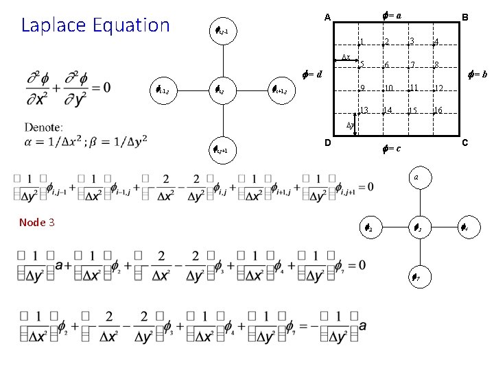
Laplace Equation f=a A fi, j-1 Dx f=d fi-1, j B fi, j fi+1, j 1 2 3 4 5 6 7 8 9 10 11 12 13 14 15 16 f=b Dy fi, j+1 D C f=c a Node 3 f 2 f 3 f 7 f 4

Laplace Equation f=a A Dx f=d Assuming the origin at D B 1 2 3 4 5 6 7 8 9 10 11 12 13 14 15 16 f=b Dy D C f=c Node No. x y x-neighbour y-neighbour 1 Δx 4Δy �� = d, 2 5, �� =a 3 3Δx 4Δy 2, 4 7, �� =a 6 2Δx 3Δy 5, 7 10, 2 9 Δx 2Δy �� = d, 10 13, 5

A One equation for each node! �� b

Laplace Equation f=a A fi, j-1 Dx f=d fi-1, j B fi, j fi+1, j 1 2 3 4 5 6 7 8 9 10 11 12 13 14 15 16 f=b Dy fi, j+1 D C f=c f 2 Node 6 f 5 f 6 f 10 f 7

Laplace Equation f=a A Dx f=d Assuming the origin at D B 1 2 3 4 5 6 7 8 9 10 11 12 13 14 15 16 f=b Dy D C f=c Node No. x y x-neighbour y-neighbour 1 Δx 4Δy �� = d, 2 5, �� =a 3 3Δx 4Δy 2, 4 7, �� =a 6 2Δx 3Δy 5, 7 10, 2 9 Δx 2Δy �� = d, 10 13, 5

A One equation for each node! �� b

Laplace Equation f=a A fi, j-1 Dx f=d fi-1, j B fi, j fi+1, j 1 2 3 4 5 6 7 8 9 10 11 12 13 14 15 16 f=b Dy fi, j+1 D C f=c f 5 Node 9 d f 9 f 13 f 10

Laplace Equation f=a A Dx f=d Assuming the origin at D B 1 2 3 4 5 6 7 8 9 10 11 12 13 14 15 16 f=b Dy D C f=c Node No. x y x-neighbour y-neighbour 1 Δx 4Δy �� = d, 2 5, �� =a 3 3Δx 4Δy 2, 4 7, �� =a 6 2Δx 3Δy 5, 7 10, 2 9 Δx 2Δy �� = d, 10 13, 5

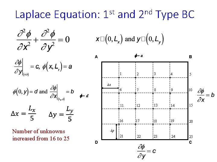
Laplace Equation: 1 st and 2 nd Type BC f=a A B 1 2 3 4 5 6 7 8 9 10 11 12 13 14 15 16 17 18 19 20 21 22 23 24 25 Dx f=d Number of unknowns increased from 16 to 25 Dy D C

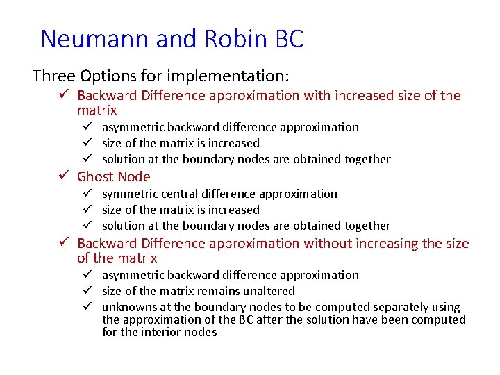
Neumann and Robin BC Three Options for implementation: ü Backward Difference approximation with increased size of the matrix ü asymmetric backward difference approximation ü size of the matrix is increased ü solution at the boundary nodes are obtained together ü Ghost Node ü symmetric central difference approximation ü size of the matrix is increased ü solution at the boundary nodes are obtained together ü Backward Difference approximation without increasing the size of the matrix ü asymmetric backward difference approximation ü size of the matrix remains unaltered ü unknowns at the boundary nodes to be computed separately using the approximation of the BC after the solution have been computed for the interior nodes

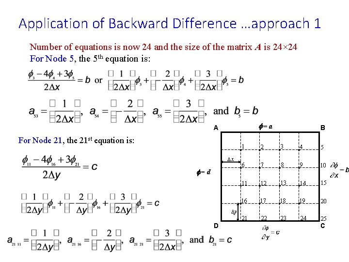
Application of Backward Difference …approach 1 Number of equations is now 24 and the size of the matrix A is 24× 24 For Node 5, the 5 th equation is: f=a A For Node 21, the 21 st equation is: Dx f=d B 1 2 3 4 5 6 7 8 9 10 11 12 13 14 15 16 17 18 19 20 21 22 23 24 25 Dy D C

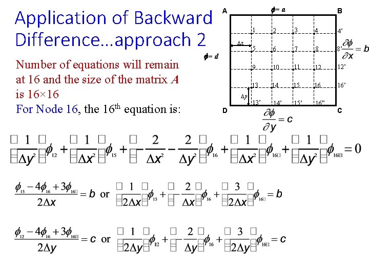
Application of Backward Difference…approach 2 Number of equations will remain at 16 and the size of the matrix A is 16× 16 For Node 16, the 16 th equation is: f=a A Dx f=d Dy D B 1 2 3 4 4’ 5 6 7 8 8’ 9 10 11 12 12’ 13 14 15 16 16’ 13’ 14’ 15’ 16” C

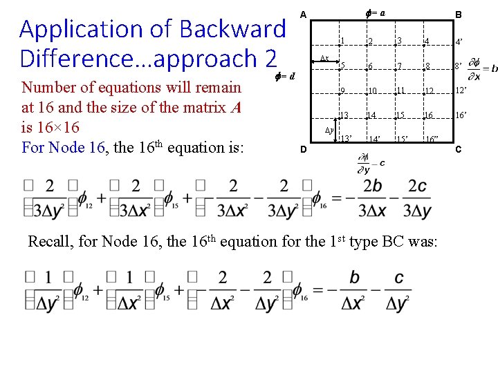
Application of Backward Difference…approach 2 Number of equations will remain at 16 and the size of the matrix A is 16× 16 For Node 16, the 16 th equation is: f=a A Dx f=d Dy D B 1 2 3 4 4’ 5 6 7 8 8’ 9 10 11 12 12’ 13 14 15 16 16’ 13’ 14’ 15’ 16” Recall, for Node 16, the 16 th equation for the 1 st type BC was: C

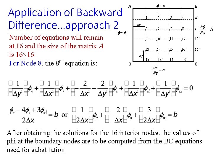
Application of Backward Difference…approach 2 Number of equations will remain at 16 and the size of the matrix A is 16× 16 For Node 8, the 8 th equation is: f=a A Dx f=d Dy B 1 2 3 4 4’ 5 6 7 8 8’ 9 10 11 12 12’ 13 14 15 16 16’ 13’ 14’ 15’ 16” D C ’ ’ ’ After obtaining the solutions for the 16 interior nodes, the values of phi at the boundary nodes are to be computed from the BC equations used for substitution!

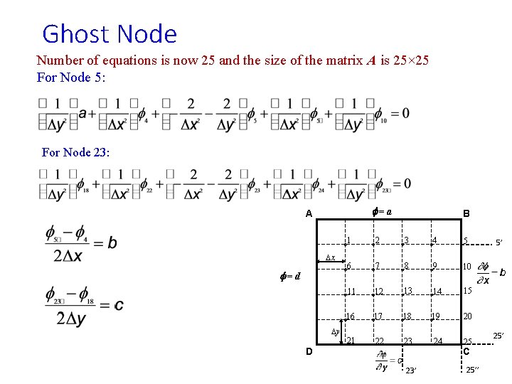
Ghost Node Number of equations is now 25 and the size of the matrix A is 25× 25 For Node 5: For Node 23: f=a A Dx f=d Dy D B 1 2 3 4 5 6 7 8 9 10 11 12 13 14 15 16 17 18 19 20 21 22 23 24 25 23’ C 25’’ 5’ 25’

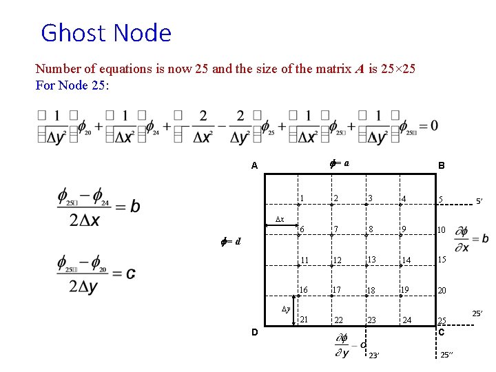
Ghost Node Number of equations is now 25 and the size of the matrix A is 25× 25 For Node 25: f=a A B 1 2 3 4 5 6 7 8 9 10 11 12 13 14 15 16 17 18 19 20 21 22 23 24 25 5’ Dx f=d Dy D C 23’ 25’

ESO 208 A: Computational Methods in Engineering Partial Differential Equation: Hyperbolic Equation Department of Civil Engineering IIT Kanpur

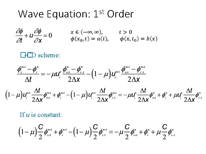
Wave Equation: 1 st Order �� -CD scheme: If u is constant:

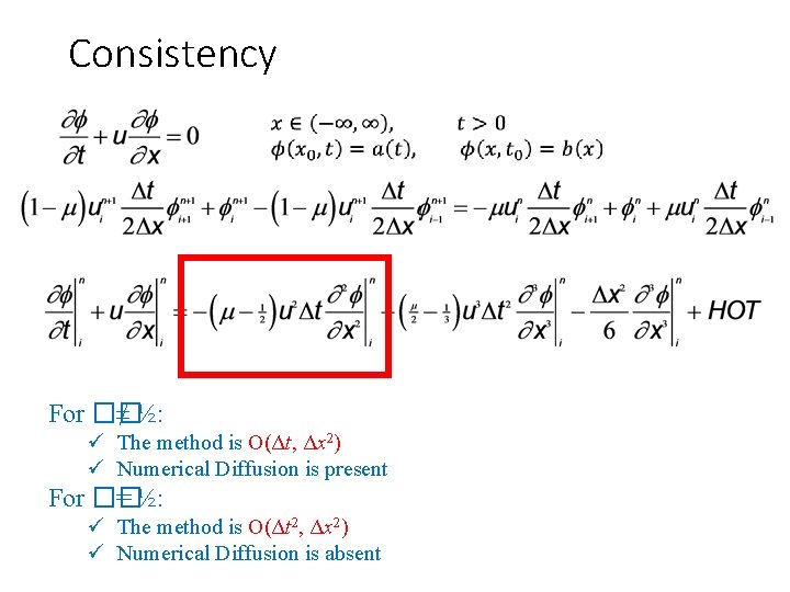
Consistency For �� ≠ ½: ü The method is O(Δt, Δx 2) ü Numerical Diffusion is present For �� = ½: ü The method is O(Δt 2, Δx 2) ü Numerical Diffusion is absent

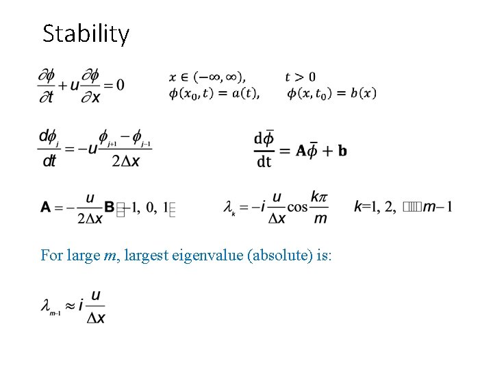
Stability For large m, largest eigenvalue (absolute) is:

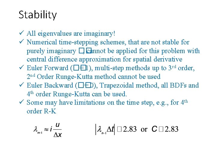
Stability ü All eigenvalues are imaginary! ü Numerical time-stepping schemes, that are not stable for purely imaginary �� , cannot be applied for this problem with central difference approximation for spatial derivative ü Euler Forward (�� = 1), multi-step methods up to 3 rd order, 2 nd Order Runge-Kutta method cannot be used ü Euler Backward (�� = 0), Trapezoidal method, all BDFs and 4 th order Runge-Kutta can be used. ü Some may have limitations on the time step, e. g. , for 4 th order R-K

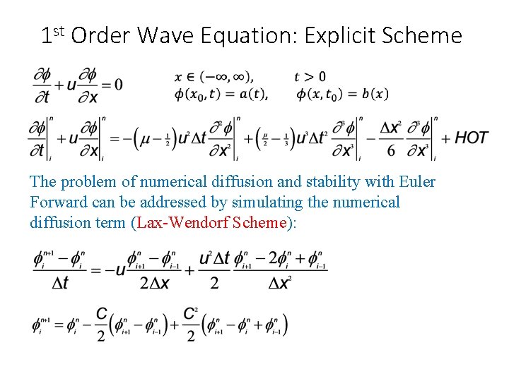
1 st Order Wave Equation: Explicit Scheme The problem of numerical diffusion and stability with Euler Forward can be addressed by simulating the numerical diffusion term (Lax-Wendorf Scheme):

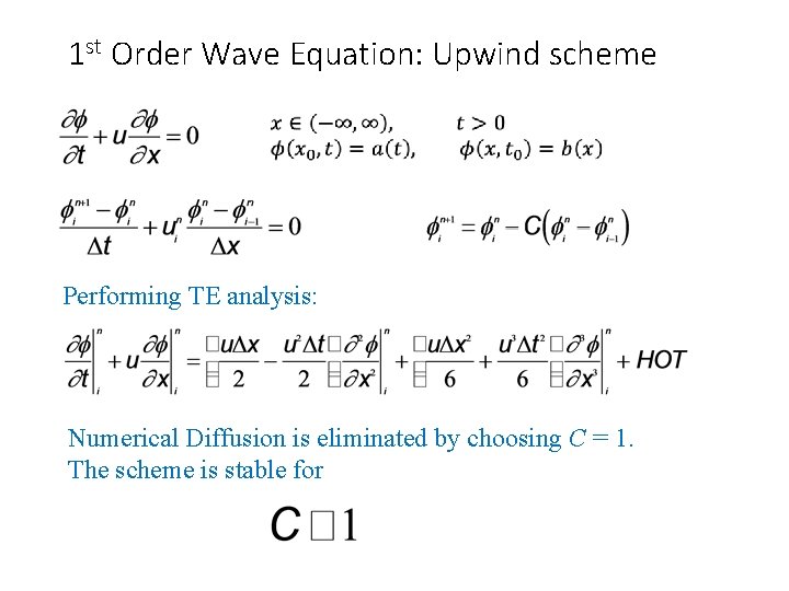
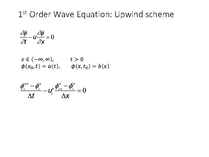
1 st Order Wave Equation: Upwind scheme Performing TE analysis: Numerical Diffusion is eliminated by choosing C = 1. The scheme is stable for

1 st Order Wave Equation: Upwind scheme

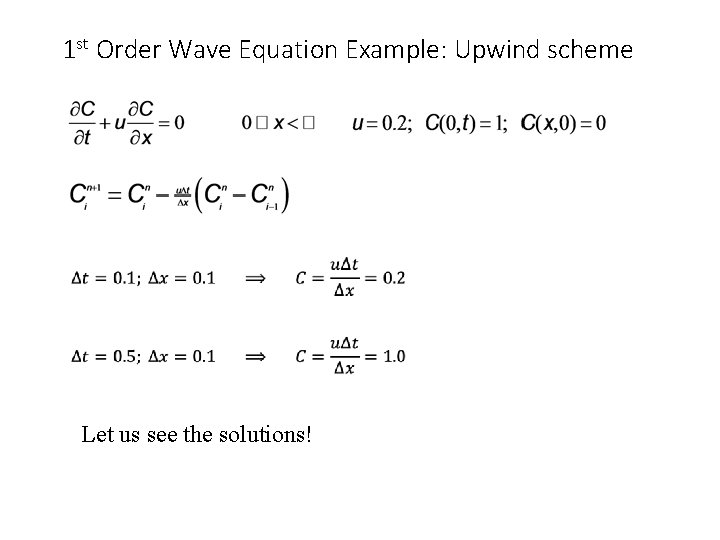
1 st Order Wave Equation Example: Upwind scheme Let us see the solutions!

Syllabus for End Sem • All topics covered in the course (40 lectures) • Roughly ~25% from pre-mid sem (could be part of postmid sem problems or as exclusive problems) • Roughly ~75% from post-mid sem Exceptions • Derivation involving local variables to derive cubic splines; numericals can be tested • Derivation of phase error in Stability problems of ODEs • Derivation of Du Fort–Frankel scheme

Consistent Attendance Missed one class/ tutorial 100% attendance 170346 KRISHAN KUMAR 170403 MUDIT KUMAR 170410 NAMAN AGRAWAL (M AGRAWAL) 170545 RAKESH KUMAR 170632 SARANSH NADDA 170739 SUNIT SHARMA 180063 AKSHAT KUMAR 180168 AVIRAL AGGARWAL 180192 BHARAT BHUSAN RATH 180360 KORAPATI AKHIL RATNA 180658 SAMPADA SINHA 180683 SAURABH JAYANT 180749 SHUBHAM GUPTA

Integrity Voluntarily gave-up their marks which were incorrectly awarded to them 170660 SHASHWAT SHUKLA 180182 AYUSHI GOYAL 180404 MANEESH P M Another student whose record I did not keep

Acknowledgements • Tutors • Teaching Assistants • LHC Staff • Professors Saumyen Guha and Shivam Tripathi • Students who regularly put up with me Good luck in end-sems! Please Use the Method Asked and Solve!