Evaluation and pricing of risk under stochastic volatility

Evaluation and pricing of risk under stochastic volatility Giacomo Bormetti Scuola Normale Superiore, Pisa

Agenda ① P versus Q: a brief overview of two branches of quantitative finance Freely inspired by http: //ssrn. com/abstract=1717163 ② The Stochastic Discount Factor The link with Asset Pricing and the Consumption. Investment optimization problem ③ An SDF perspective over P and Q Realizing smiles and quantiles

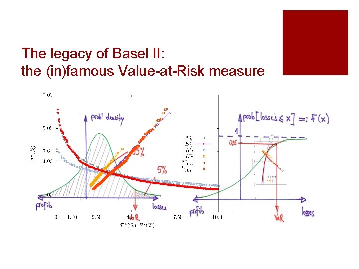
Risk and portfolio management: the P world a. Risk and portfolio management aims at modelling the probability distribution of the market prices at a given future investment horizon b. The probability distribution P must be estimated from available information. A major component of this information set is the past dynamics of prices, which are monitored at discrete time intervals and stored in the form of time series c. Estimation represents the main quantitative challenge in the P world

The legacy of Basel II: the (in)famous Value-at-Risk measure

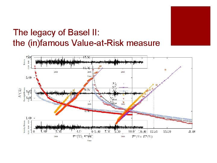
The legacy of Basel II: the (in)famous Value-at-Risk measure

Derivatives pricing: the Q world a. The goal of derivatives pricing is to determine the fair price of a given security in terms of the underlying securities whose price is determined by the law of supply and demand. b. The risk-neutral probability Q and the real probability P associate different weights to the same possible outcomes for the same financial variables. The transition from one set of probability weights to the other defines the so-called risk-premium. c. Calibration is one of the main challenges of the Q world. d. Forward-looking measure.

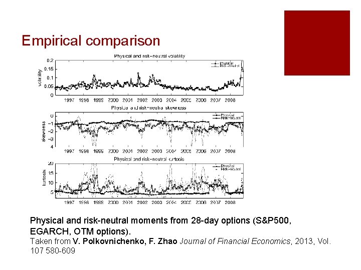
Empirical comparison Physical and risk-neutral moments from 28 -day options (S&P 500, EGARCH, OTM options). Taken from V. Polkovnichenko, F. Zhao Journal of Financial Economics, 2013, Vol. 107 580 -609

The Stochastic Discount Factor ① We now study the consumption-investment optimization problem of an agent maximizing an intertemporal utility criterion ② The optimality conditions implied by agents optimal intertemporal choices show the existence of a universal random variable, the stochastic discount factor (SDF), such that asset prices are expectations of contingent payoffs scaled by the SDF.

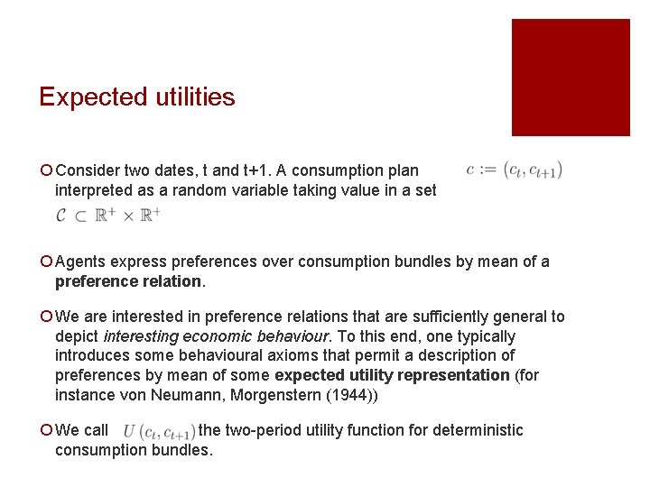
Expected utilities ¡ Consider two dates, t and t+1. A consumption plan interpreted as a random variable taking value in a set can be ¡ Agents express preferences over consumption bundles by mean of a preference relation. ¡ We are interested in preference relations that are sufficiently general to depict interesting economic behaviour. To this end, one typically introduces some behavioural axioms that permit a description of preferences by mean of some expected utility representation (for instance von Neumann, Morgenstern (1944)) ¡ We call the two-period utility function for deterministic consumption bundles.

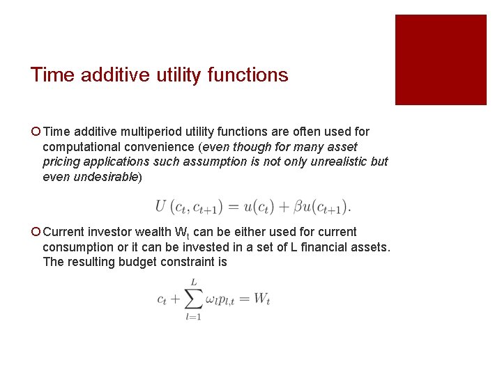
Time additive utility functions ¡ Time additive multiperiod utility functions are often used for computational convenience (even though for many asset pricing applications such assumption is not only unrealistic but even undesirable) ¡ Current investor wealth Wt can be either used for current consumption or it can be invested in a set of L financial assets. The resulting budget constraint is

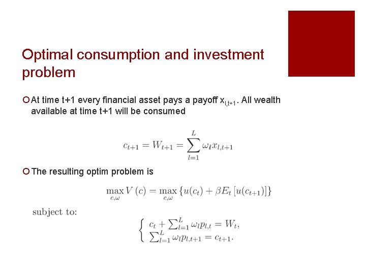
Optimal consumption and investment problem ¡ At time t+1 every financial asset pays a payoff xl, t+1. All wealth available at time t+1 will be consumed ¡ The resulting optim problem is

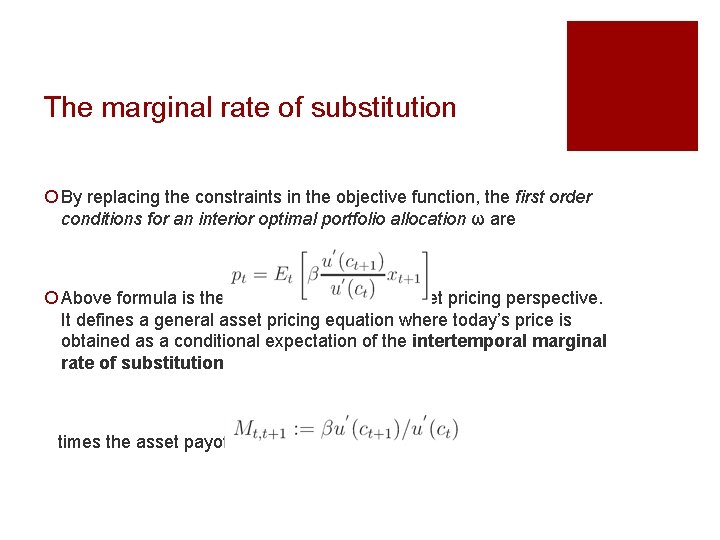
The marginal rate of substitution ¡ By replacing the constraints in the objective function, the first order conditions for an interior optimal portfolio allocation ω are ¡ Above formula is the key formula from our asset pricing perspective. It defines a general asset pricing equation where today’s price is obtained as a conditional expectation of the intertemporal marginal rate of substitution times the asset payoff.

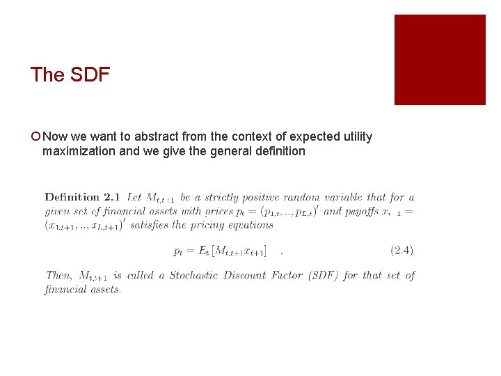
The SDF ¡ Now we want to abstract from the context of expected utility maximization and we give the general definition

The fundamental theorem of asset pricing ① Which general economic assumptions may ensure the existence of a SDF? The economic content of the existence of a positive SDF is the absence of arbitrage opportunities in the market ② Under which conditions is the SDF unique, when it exists? The SDF is unique when markets are complete

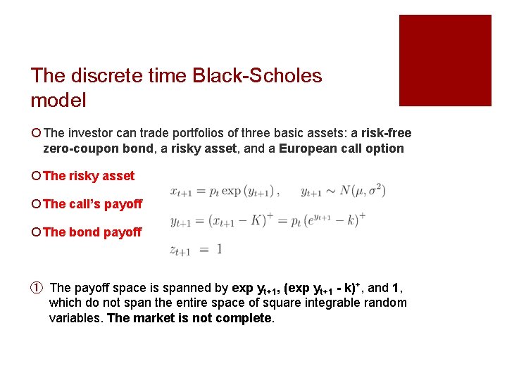
The discrete time Black-Scholes model ¡ The investor can trade portfolios of three basic assets: a risk-free zero-coupon bond, a risky asset, and a European call option ¡ The risky asset ¡ The call’s payoff ¡ The bond payoff ① The payoff space is spanned by exp yt+1, (exp yt+1 - k)+, and 1, which do not span the entire space of square integrable random variables. The market is not complete.

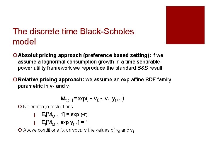
The discrete time Black-Scholes model ¡ Absolut pricing approach (preference based setting): if we assume a lognormal consumption growth in a time separable power utility framework we reproduce the standard B&S result ¡ Relative pricing approach: we assume an exp affine SDF family parametric in v 0 and v 1 Mt, t+1=exp( - v 0 - v 1 yt+1 ) ¡ No arbitrage restrictions ¡ ¡ Et[Mt, t+1 1] = exp (-r) Et[Mt, t+1 exp yt+1] = 1 ¡ Above conditions fix univocally the values of v 0 and v 1

Realizing smiles and quantiles ¡ An SDF perspective over Q and P ¡ Work in progress with Adam A. Majewskij and Fulvio Corsi

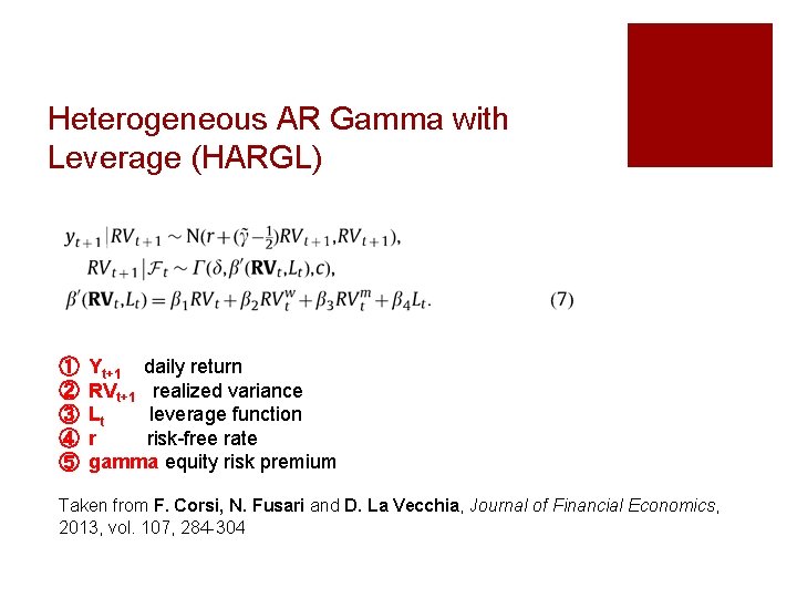
Heterogeneous AR Gamma with Leverage (HARGL) ① ② ③ ④ ⑤ Yt+1 daily return RVt+1 realized variance Lt leverage function r risk-free rate gamma equity risk premium Taken from F. Corsi, N. Fusari and D. La Vecchia, Journal of Financial Economics, 2013, vol. 107, 284 -304

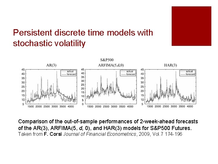
Persistent discrete time models with stochastic volatility Comparison of the out-of-sample performances of 2 -week-ahead forecasts of the AR(3), ARFIMA(5, d, 0), and HAR(3) models for S&P 500 Futures. Taken from F. Corsi Journal of Financial Econometrics, 2009, Vol. 7 174 -196

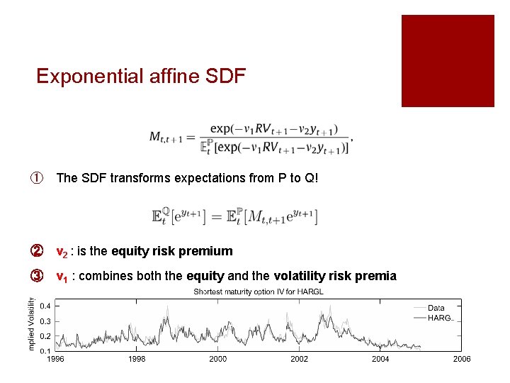
Exponential affine SDF ① The SDF transforms expectations from P to Q! ② v 2 : is the equity risk premium ③ v 1 : combines both the equity and the volatility risk premia

Realizing quantiles ¡ Musil’s imaginary bridge You begin with ordinary solid numbers, representing measures of length or weight or something else that’s quite tangible - at any rate, they’re real numbers. And at the end you have real numbers. But these two lots of real numbers are connected by something that simply doesn’t exist. Isn’t that like a bridge where the piles are there only at the beginning and at the end, with none in the middle, and yet one crosses it just as surely and safely as if the whole of it were there? That sort of operation makes me feel a bit giddy R. Musil, Young Törless

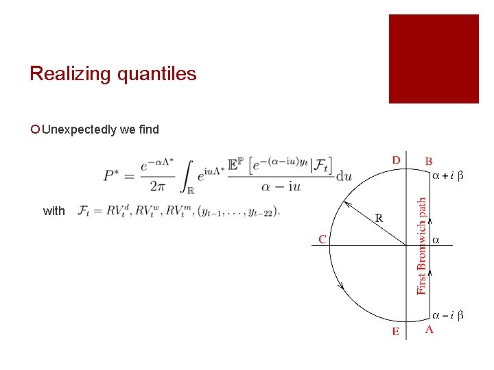
Realizing quantiles ¡ Unexpectedly we find with