Environmental and Exploration Geophysics II Gravity Methods IV

Environmental and Exploration Geophysics II Gravity Methods (IV) tom. h. wilson tom. wilson@mail. wvu. edu Department of Geology and Geography West Virginia University Morgantown, WV Tom Wilson, Department of Geology and Geography

What physical characteristics of the observation point and it’s surroundings influence the observed acceleration of gravity? Tom Wilson, Department of Geology and Geography

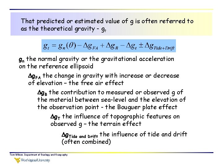
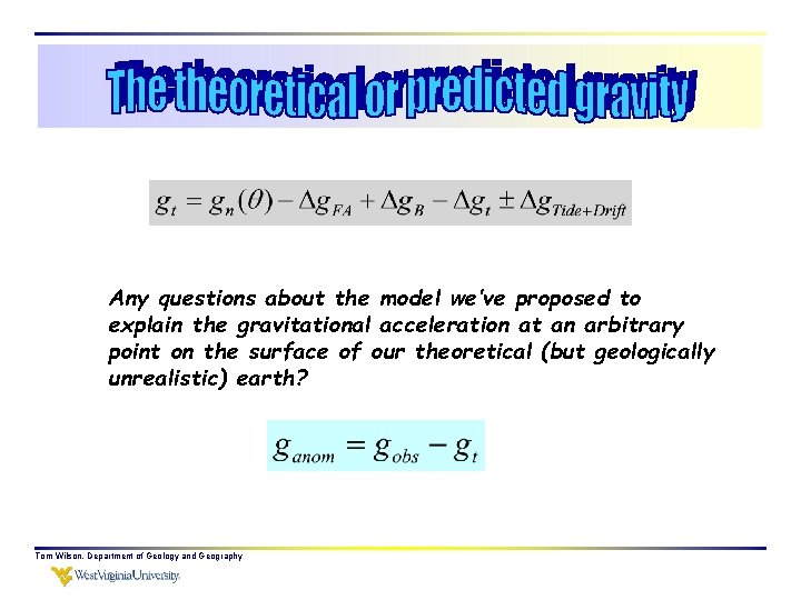
That predicted or estimated value of g is often referred to as theoretical gravity - gt gn the normal gravity or the gravitational acceleration on the reference ellipsoid g. FA the change in gravity with increase or decrease of elevation – the free air effect g. B the contribution to measured or observed g of the material between sea-level and the elevation of the observation point - the Bouguer plate effect g. T the influence of topographic features on observed g – the terrain effect g. Tide and Drift the influence of tide and drift (often combined) Tom Wilson, Department of Geology and Geography

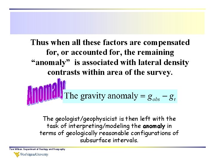
Thus when all these factors are compensated for, or accounted for, the remaining “anomaly” is associated with lateral density contrasts within area of the survey. The geologist/geophysicist is then left with the task of interpreting/modeling the anomaly in terms of geologically reasonable configurations of subsurface intervals. Tom Wilson, Department of Geology and Geography

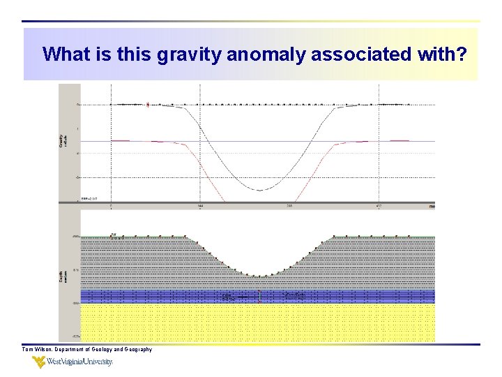
What is this gravity anomaly associated with? Tom Wilson, Department of Geology and Geography

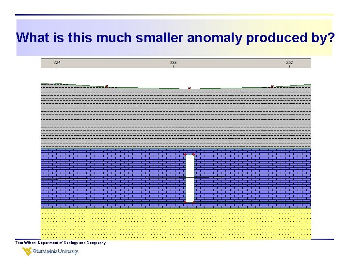
What is this much smaller anomaly produced by? Tom Wilson, Department of Geology and Geography

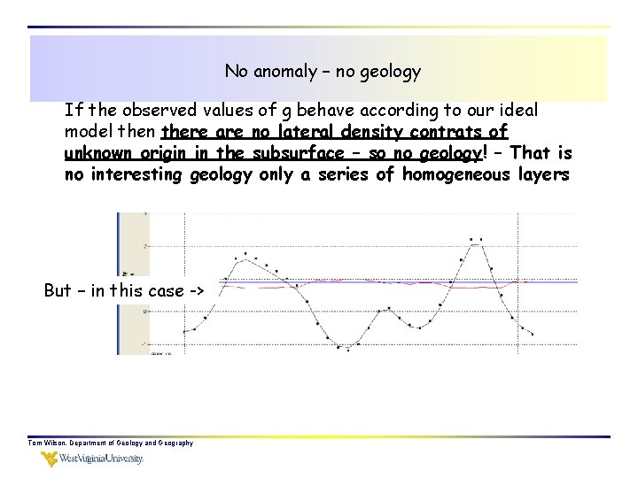
No anomaly – no geology If the observed values of g behave according to our ideal model then there are no lateral density contrats of unknown origin in the subsurface – so no geology! – That is no interesting geology only a series of homogeneous layers But – in this case -> Tom Wilson, Department of Geology and Geography

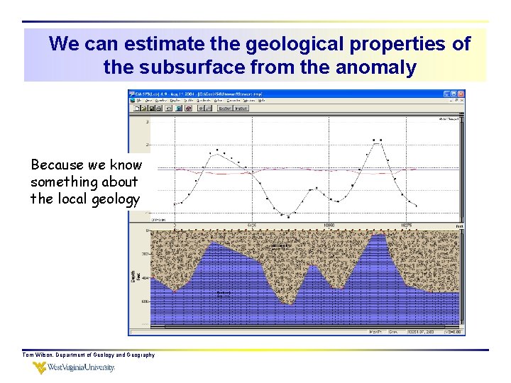
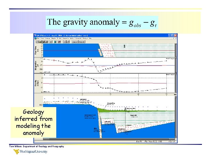
We can estimate the geological properties of the subsurface from the anomaly Because we know something about the local geology Tom Wilson, Department of Geology and Geography

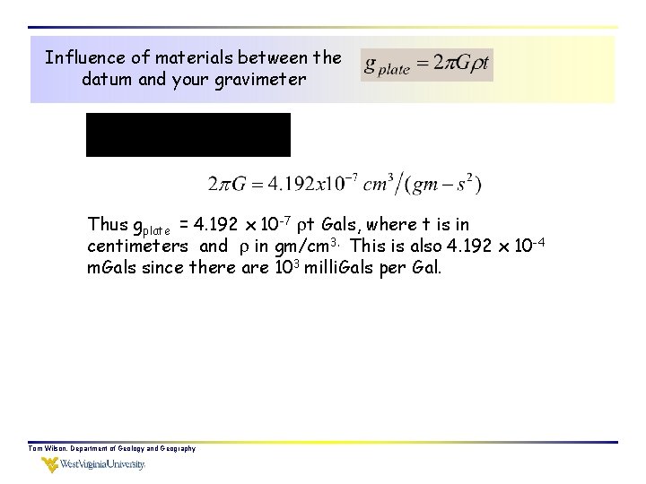
Influence of materials between the datum and your gravimeter Thus gplate = 4. 192 x 10 -7 t Gals, where t is in centimeters and in gm/cm 3. This is also 4. 192 x 10 -4 m. Gals since there are 103 milli. Gals per Gal. Tom Wilson, Department of Geology and Geography

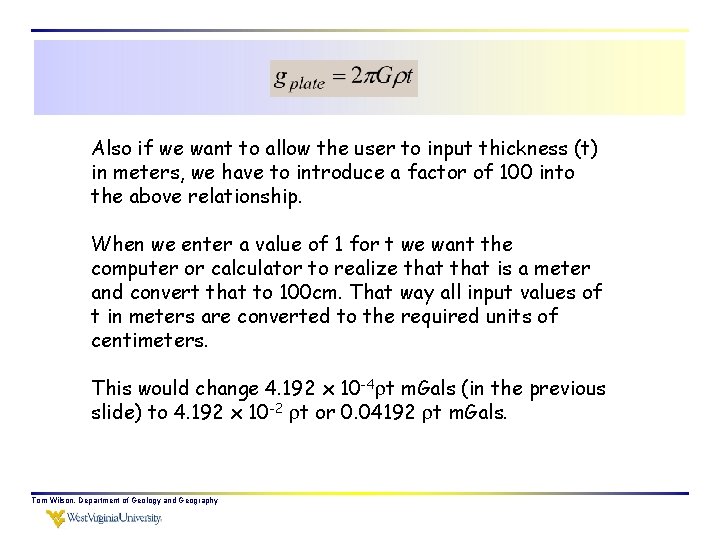
Also if we want to allow the user to input thickness (t) in meters, we have to introduce a factor of 100 into the above relationship. When we enter a value of 1 for t we want the computer or calculator to realize that is a meter and convert that to 100 cm. That way all input values of t in meters are converted to the required units of centimeters. This would change 4. 192 x 10 -4 t m. Gals (in the previous slide) to 4. 192 x 10 -2 t or 0. 04192 t m. Gals. Tom Wilson, Department of Geology and Geography

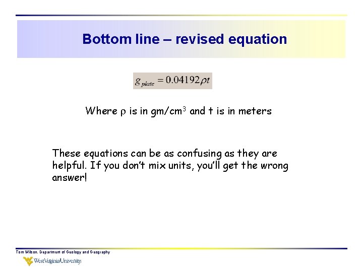
Bottom line – revised equation Where is in gm/cm 3 and t is in meters These equations can be as confusing as they are helpful. If you don’t mix units, you’ll get the wrong answer! Tom Wilson, Department of Geology and Geography

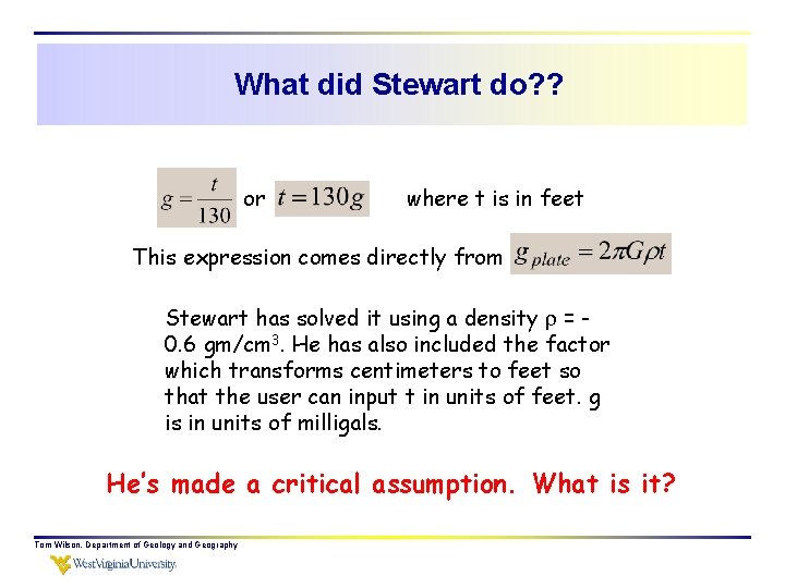
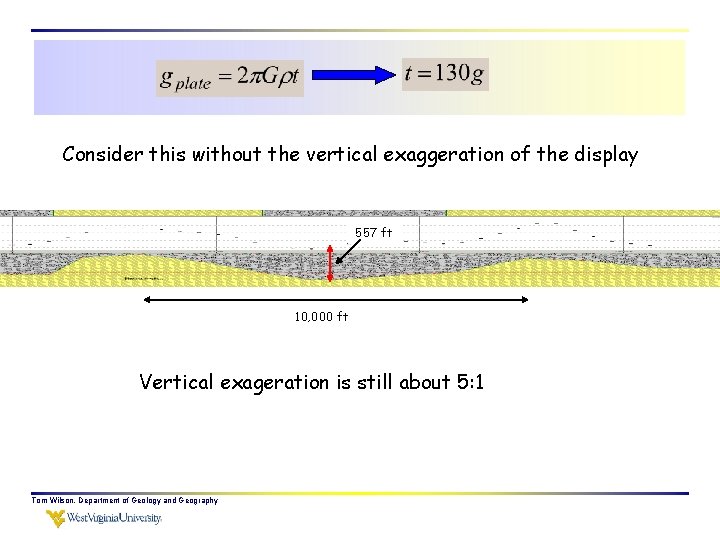
What did Stewart do? ? or where t is in feet This expression comes directly from Stewart has solved it using a density = 0. 6 gm/cm 3. He has also included the factor which transforms centimeters to feet so that the user can input t in units of feet. g is in units of milligals. He’s made a critical assumption. What is it? Tom Wilson, Department of Geology and Geography

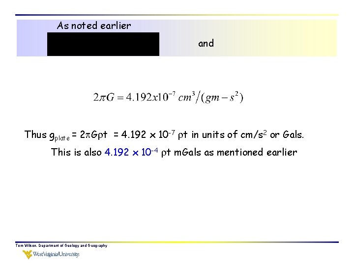
Consider this without the vertical exaggeration of the display 557 ft 10, 000 ft Vertical exageration is still about 5: 1 Tom Wilson, Department of Geology and Geography

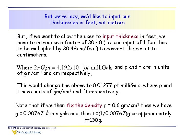
As noted earlier and Thus gplate = 2 G t = 4. 192 x 10 -7 t in units of cm/s 2 or Gals. This is also 4. 192 x 10 -4 t m. Gals as mentioned earlier Tom Wilson, Department of Geology and Geography

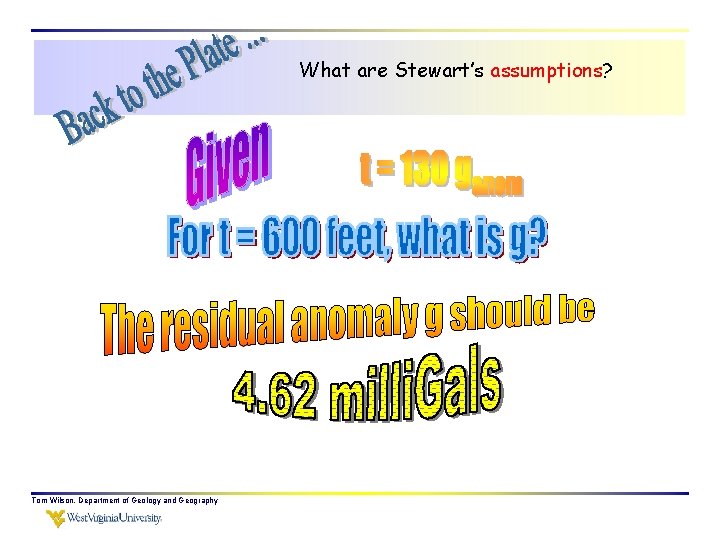
But we’re lazy, we’d like to input our thicknesses in feet, not meters But, if we want to allow the user to input thickness in feet, we have to introduce a factor of 30. 48 (i. e. our input of 1 foot has to be multiplied by 30. 48 cm/foot) to convert the result to centimeters. of gm/cm 3 and cm respectively, and t are in units This would change the above to 0. 01277 t milli. Gals, where and t have units of gm/cm 3 and ft respectively. Note that if we then fix the density = 0. 6 gm/cm 3 then we have g = 0. 00767 t in mgals and thus t =(1/0. 00767)g or approximately Tom Wilson, Department of Geology and Geography t=130 g.

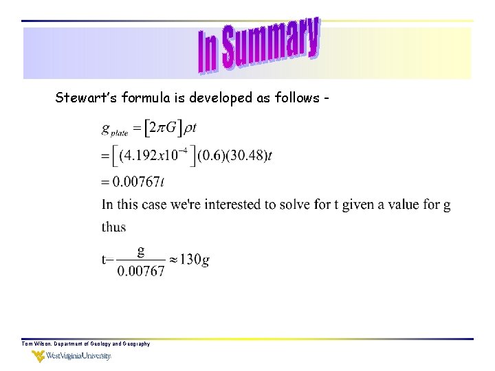
Stewart’s formula is developed as follows - Tom Wilson, Department of Geology and Geography

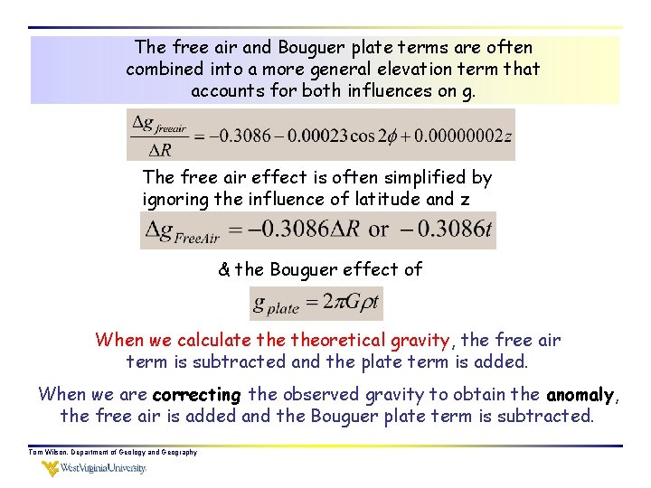
The free air and Bouguer plate terms are often combined into a more general elevation term that accounts for both influences on g. The free air effect is often simplified by ignoring the influence of latitude and z & the Bouguer effect of When we calculate theoretical gravity, the free air term is subtracted and the plate term is added. When we are correcting the observed gravity to obtain the anomaly, the free air is added and the Bouguer plate term is subtracted. Tom Wilson, Department of Geology and Geography

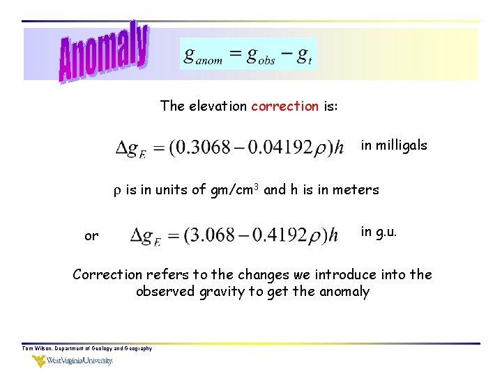
The elevation correction is: in milligals is in units of gm/cm 3 and h is in meters or in g. u. Correction refers to the changes we introduce into the observed gravity to get the anomaly Tom Wilson, Department of Geology and Geography

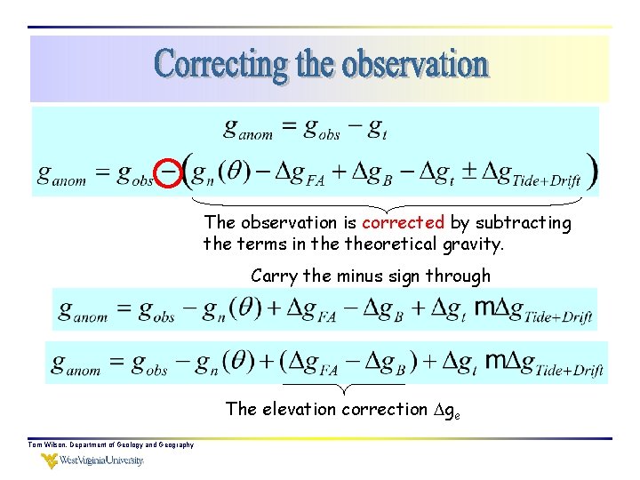
The observation is corrected by subtracting the terms in theoretical gravity. Carry the minus sign through The elevation correction ge Tom Wilson, Department of Geology and Geography

What are Stewart’s assumptions? Tom Wilson, Department of Geology and Geography

Tom Wilson, Department of Geology and Geography

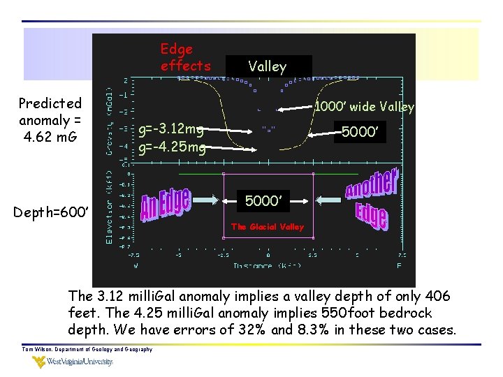
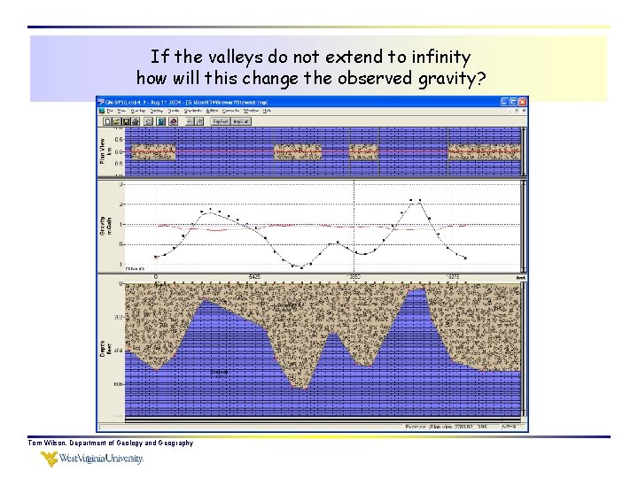
Edge effects Predicted anomaly = 4. 62 m. G Valley 1000’ wide Valley g=-3. 12 mg g=-4. 25 mg Depth=600’ 5000’ The Glacial Valley The 3. 12 milli. Gal anomaly implies a valley depth of only 406 feet. The 4. 25 milli. Gal anomaly implies 550 foot bedrock depth. We have errors of 32% and 8. 3% in these two cases. Tom Wilson, Department of Geology and Geography

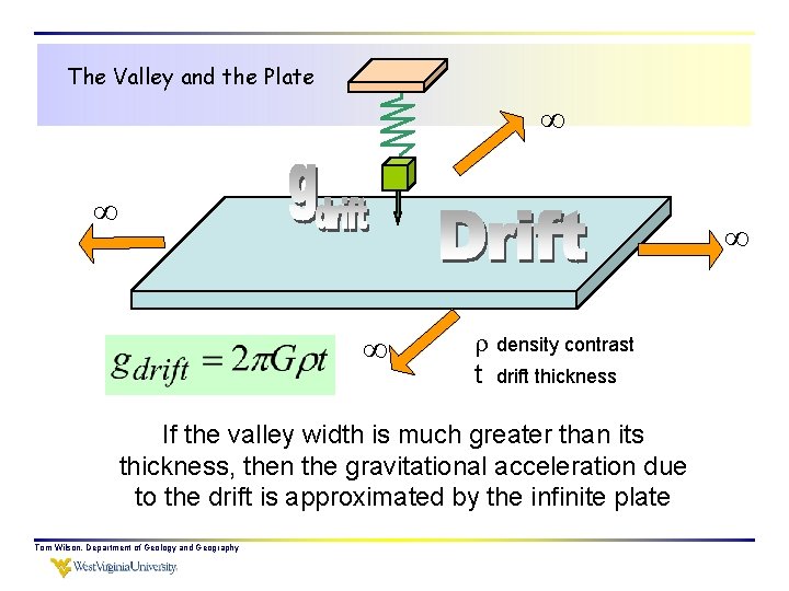
The Valley and the Plate density contrast t drift thickness If the valley width is much greater than its thickness, then the gravitational acceleration due to the drift is approximated by the infinite plate Tom Wilson, Department of Geology and Geography

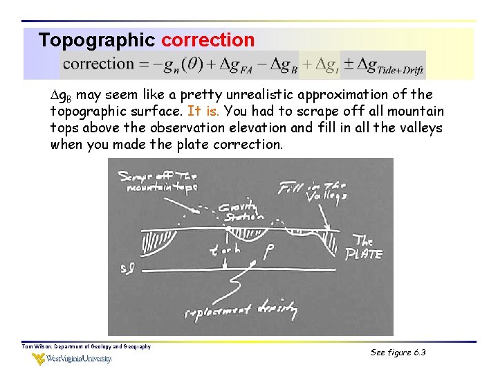
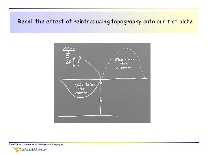
Topographic correction g. B may seem like a pretty unrealistic approximation of the topographic surface. It is. You had to scrape off all mountain tops above the observation elevation and fill in all the valleys when you made the plate correction. Tom Wilson, Department of Geology and Geography See figure 6. 3

Recall the effect of reintroducing topography onto our flat plate Tom Wilson, Department of Geology and Geography

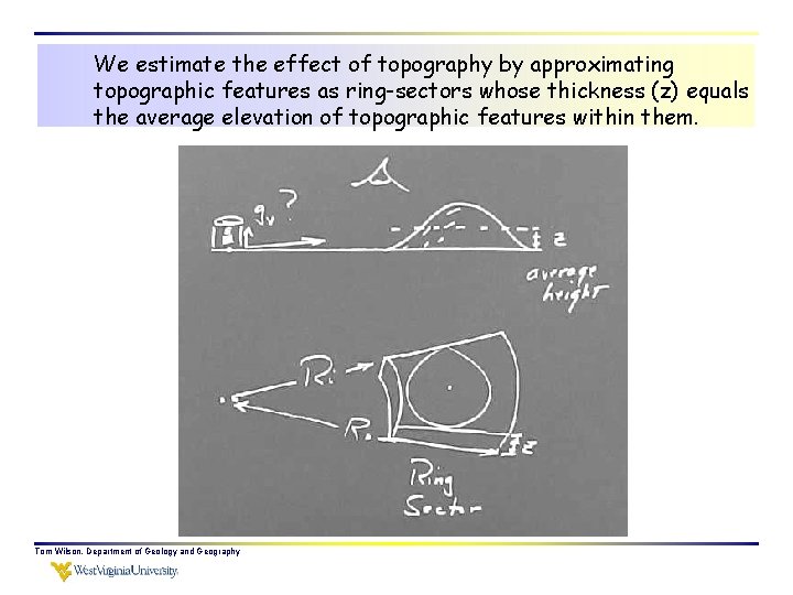
We estimate the effect of topography by approximating topographic features as ring-sectors whose thickness (z) equals the average elevation of topographic features within them. Tom Wilson, Department of Geology and Geography

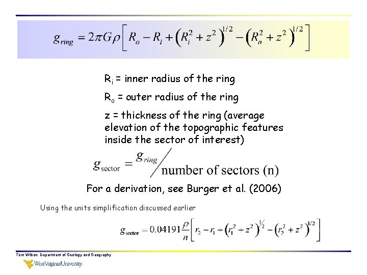
Ri = inner radius of the ring Ro = outer radius of the ring z = thickness of the ring (average elevation of the topographic features inside the sector of interest) For a derivation, see Burger et al. (2006) Using the units simplification discussed earlier Tom Wilson, Department of Geology and Geography

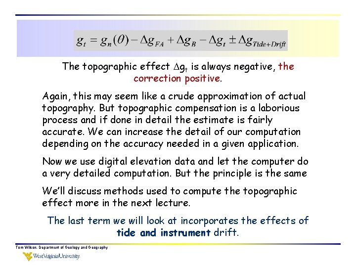
The topographic effect gt is always negative, the correction positive. Again, this may seem like a crude approximation of actual topography. But topographic compensation is a laborious process and if done in detail the estimate is fairly accurate. We can increase the detail of our computation depending on the accuracy needed in a given application. Now we use digital elevation data and let the computer do a very detailed computation. But the principle is the same We’ll discuss methods used to compute the topographic effect more in the next lecture. The last term we will look at incorporates the effects of tide and instrument drift. Tom Wilson, Department of Geology and Geography

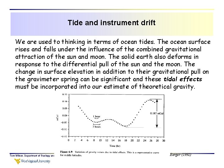
Tide and instrument drift We are used to thinking in terms of ocean tides. The ocean surface rises and falls under the influence of the combined gravitational attraction of the sun and moon. The solid earth also deforms in response to the differential pull of the sun and the moon. The change in surface elevation in addition to their gravitational pull on the gravimeter spring can be significant and these tidal effects must be incorporated into our estimate of theoretical gravity. Tom Wilson, Department of Geology and Geography Berger (1992)

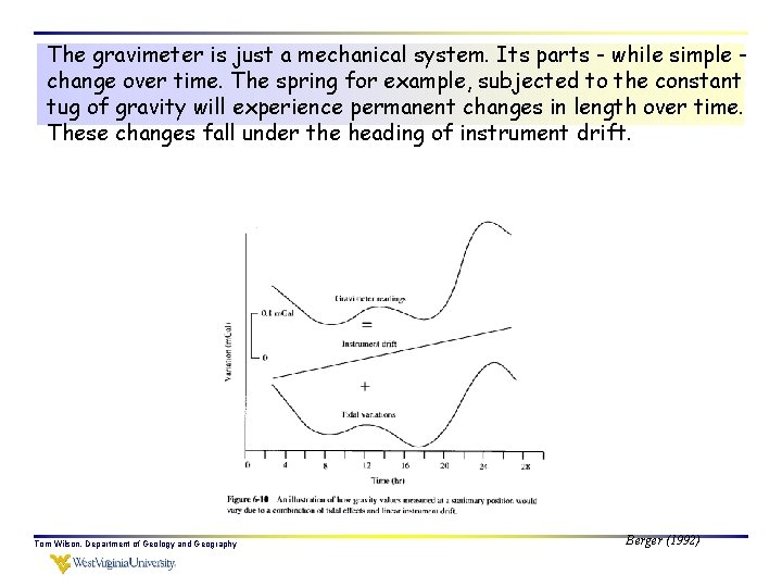
The gravimeter is just a mechanical system. Its parts - while simple change over time. The spring for example, subjected to the constant tug of gravity will experience permanent changes in length over time. These changes fall under the heading of instrument drift. Tom Wilson, Department of Geology and Geography Berger (1992)

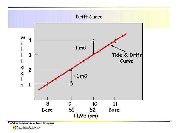
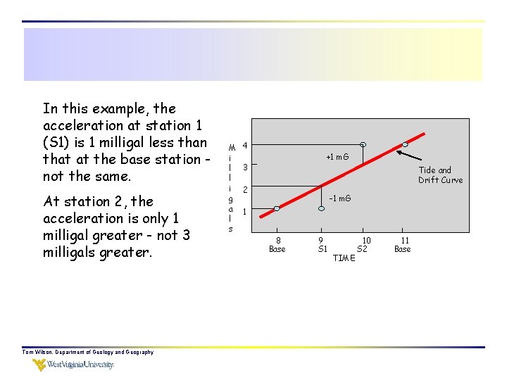
In general the influence of tide and drift on theoretical gravity is estimated by direct and repeated measurement of gravitational acceleration at the same place (a base station) over and over again, throughout the duration of your survey. Usually during a survey a base station is reoccupied every couple hours or so. The “drift curve” is constructed from these measurements and measurements of acceleration made at other stations are corrected relative to the drift curve. Tom Wilson, Department of Geology and Geography

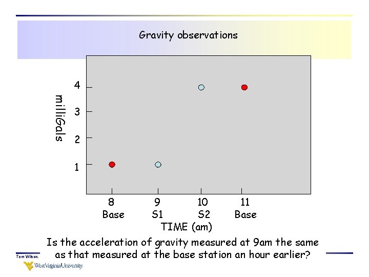
Gravity observations 4 milli. Gals 3 2 1 8 Base 9 10 11 S 2 Base TIME (am) Is the acceleration of gravity measured at 9 am the same as that measured at the base station an hour earlier? Tom Wilson, Department of Geology and Geography

Drift Curve M i l l i g a l s 4 +1 m. G Tide & Drift Curve 3 2 -1 m. G 1 8 Base Tom Wilson, Department of Geology and Geography 9 10 S 1 S 2 TIME (am) 11 Base

In this example, the acceleration at station 1 (S 1) is 1 milligal less than that at the base station not the same. At station 2, the acceleration is only 1 milligal greater - not 3 milligals greater. Tom Wilson, Department of Geology and Geography M i l l i g a l s 4 +1 m. G 3 Tide and Drift Curve 2 -1 m. G 1 8 Base 9 S 1 TIME 10 S 2 11 Base

Any questions about the model we’ve proposed to explain the gravitational acceleration at an arbitrary point on the surface of our theoretical (but geologically unrealistic) earth? Tom Wilson, Department of Geology and Geography

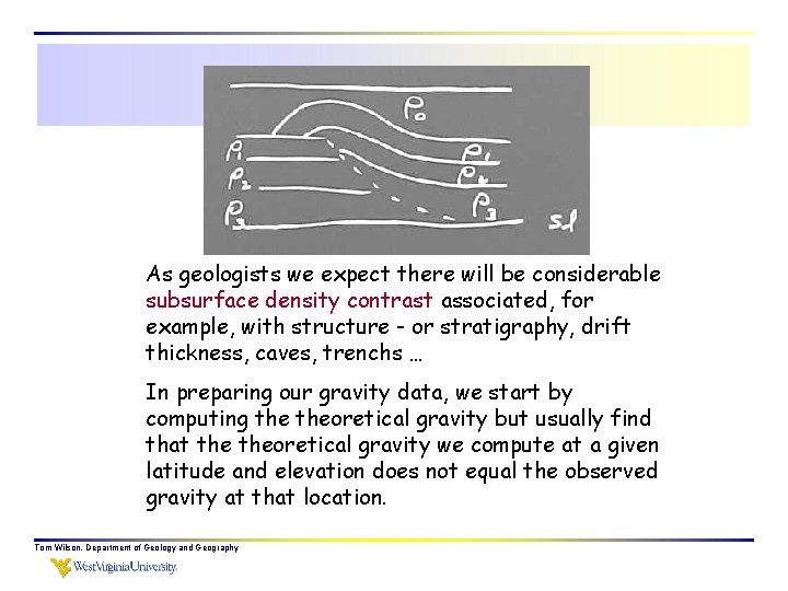
As geologists we expect there will be considerable subsurface density contrast associated, for example, with structure - or stratigraphy, drift thickness, caves, trenchs … In preparing our gravity data, we start by computing theoretical gravity but usually find that theoretical gravity we compute at a given latitude and elevation does not equal the observed gravity at that location. Tom Wilson, Department of Geology and Geography

An anomaly exists - and therein lies the geology. Geology inferred from modeling the anomaly Tom Wilson, Department of Geology and Geography

Items on the list …. • Turn in your gravity paper summaries (Tuesday, Nov. 15 th). • Any questions about problems 6. 1 – 6. 3. They will be also be due. Tuesday, Nov. 15 th. • Gravity Lab will be due on Nov. 17 th. We will clear up any questions you have about the gravity lab in the next couple lectures. • Review the remainder of the chapter 6 (past page 378). Tom Wilson, Department of Geology and Geography

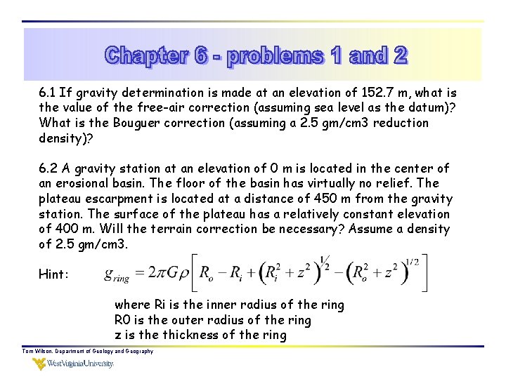
6. 1 If gravity determination is made at an elevation of 152. 7 m, what is the value of the free-air correction (assuming sea level as the datum)? What is the Bouguer correction (assuming a 2. 5 gm/cm 3 reduction density)? 6. 2 A gravity station at an elevation of 0 m is located in the center of an erosional basin. The floor of the basin has virtually no relief. The plateau escarpment is located at a distance of 450 m from the gravity station. The surface of the plateau has a relatively constant elevation of 400 m. Will the terrain correction be necessary? Assume a density of 2. 5 gm/cm 3. Hint: where Ri is the inner radius of the ring R 0 is the outer radius of the ring z is the thickness of the ring Tom Wilson, Department of Geology and Geography

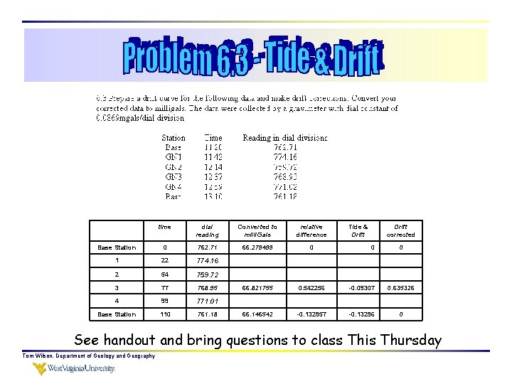
time dial reading Converted to milli. Gals relative difference Tide & Drift corrected Base Station 0 762. 71 66. 279499 0 1 22 774. 16 2 54 759. 72 3 77 768. 95 66. 821755 0. 542256 -0. 09307 0. 635326 4 99 771. 01 Base Station 110 761. 18 66. 146542 -0. 132957 -0. 13296 0 0 0 See handout and bring questions to class This Thursday Tom Wilson, Department of Geology and Geography

If the valleys do not extend to infinity how will this change the observed gravity? Tom Wilson, Department of Geology and Geography