Environmental and Exploration Geophysics II Gravity Methods II

Environmental and Exploration Geophysics II Gravity Methods (II) tom. h. wilson tom. wilson@mail. wvu. edu Department of Geology and Geography West Virginia University Morgantown, WV

To conceptualize the dependence of gravitational acceleration on various factors, we usually write g as a sum of different influences or contributions. These are -

gn the normal gravity of the gravitational acceleration on the reference ellipsoid g. FA the elevation or free air effect g. B the Bouguer plate effect or the contribution to measured or observed g of the material between sealevel and the elevation of the observation point g. T the effect of terrain on the observed g g. Tide and Drift the effects of tide and drift (often combined) These different terms can be combined into an expression which is equivalent to a prediction of what the acceleration should be at a particular point on the surface of a homogeneous earth.

Thus when all these factors are compensated for, or accounted for, the remaining “anomaly” is associated with lateral density contrasts within area of the survey. The geologist/geophysicist is then left with the task of interpreting/modeling the anomaly in terms of geologically reasonable configurations of subsurface intervals.

That predicted or estimated value of g is often referred to as theoretical gravity - gt If the observed values of g behave according to this ideal model then there is no geology! - i. e. there is no lateral heterogeneity. The geology would be fairly uninteresting - a layer cake. . . We’ll come back to this idea later, but for now let’s develop a little better understanding of the individual terms in this expression.

Consider individual terms in more detail From our discussion last period you know there are several reasons why g may differ from one point to another on the earth’s surface. 1) The earth is an oblate spheroid, and if we were to walk from the equator to the poles we would go down hill over 21 kilometers. We would be 21. 4 kilometers closer to the center of the earth at the poles. The variation in earth radius is primarily a function of latitude. 2) In addition to that we have another latitude dependant effect - centrifugal acceleration.

Let’s consider the effects of centrifugal acceleration. The velocity of a point on the earth’s equator as it rotates about the earth’s axis is ~ 1522 f/s.

What is the centrifugal acceleration at the equator? Although that acceleration is small, if it were maintained, you would drift 0. 4 meters in 5 seconds 1. 65 meters in 10 seconds Travel the average distance to the moon in 1. 74 days

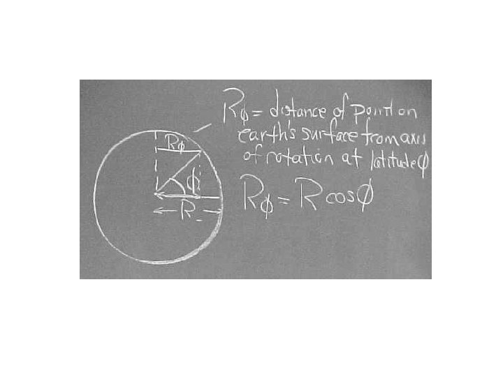
Note that as latitude changes, R in the expression does not refer to the earth’s radius, but to the distance from a point on the earth’s surface to the earth’s axis of rotation. This distance decreases with increasing latitude and becomes 0 at the poles.

Latitude Effects The combined effects of the earth’s shape and centrifugal acceleration are represented as a function of latitude ( ). The formula below was adopted as a standard by the International Association of Geodesy in 1967. The formula is referred to as the Geodetic Reference System formula of 1967 or GRS 67 See page 357 Burger et al. 2006

What is a gravity unit (otherwise known as gu)? Milli. Gals are 10 -5 m/sec 2 The milli. Gal is referenced to the Gal. In recent years, the gravity unit has become popular, largely because it’s reference is to meters/sec 2 i. e. 10 -6 m/sec 2 or 1 micrometer/sec 2.

The gradient of this effect is This is a useful expression, since you need only go through the calculation of GRS 67 once in a particular survey area. All other estimates of gn can be made by adjusting the value according to the above formula. The accuracy of your survey can be affected by an imprecise knowledge of one’s actual latitude. The above formula reveals that an error of 1 mile in latitude translates into an error of 1. 31 milligals (13. 1 gu) at a latitude of 45 o (in Morgantown, this gradient is 10. 8 gu/mile). The accuracy you need in your position latitude depends in a practical sense on the change in acceleration you are trying to detect.

The difference in g from equator to pole is approximately 5186 milligals. The variation in the middle latitudes is approximately 1. 31 milligals per mile (i. e. sin (2 ) = 1). Again, this represents the combined effects of centrifugal acceleration and polar flattening.

Free air term The next term in our expression of theoretical gravity is g. FA - the free air term In our earlier discussion we showed that dg/d. R could be approximated as -2 g/R. Using an average radius for the earth this turned out to be about 0. 3081 milligals/m (about 3 gu).

When the variations of g with latitude are considered in this estimate one finds that Where z is the elevation above sea-level. The influence of variations in z is actually quite small and generally ignored (see next slide). i. e. for most practical applications g=-0. 3086 R milligals/m Berger et al. Formula 6. 14, p 359

Free Air Effect From Burger et al. As the above plot reveals, the variations in dg/d. R, extend from 0. 3089 at the equator to 0. 3083 at the poles. In the middle latitude areas such as Morgantown, the value 0. 3086 is often used. Note that the effect of elevation is ~ 2/100, 000 th milligal (or 2/100 ths of a microgal) for 1000 meter elevation.

From Burger et al. The variation of dg/d. R with elevation - as you can see in the above graph - is quite small.

Bouguer Plate Term Next we estimate the term g. B - the Bouguer plate term. This term estimates the contribution to theoretical gravity of the material between the station elevation and sea level. We have estimated how much the acceleration will be reduced by an increase in elevation. We have reduced our estimate accordingly. But now, we need to increase our estimate to incorporate the effect of materials beneath us. First we consider the plate effect from a conceptual point of view and then we will go through the mathematical description of this effect.

We don’t have to have any geologic complexity between the measurement point and sea level. GRS 67 makes predictions (gn) of g on the reference surface (i. e. sea level). If we want to compare our observations to predictions we have to account for the fact that at our observation point g will be different from GRS 67 not only because we are at some elevation h above the reference surface but also because there is additional mass between the observation point and the reference surface.

V To determine the effect of the plate on g we must sum together the contributions of volume elements over the infinite extent of the plate.

t onen t p m n co ical of dista t r e V t ass m men m e l o e r f e volum Acceleration due to mass of volume element directly beneath the gravimeter

To do this we evaluate Newton’s universal law of gravitation in its integral form.

We’ll solve this equation by doing the integrations one variable at a time. We start with integration along the x axis. This turns out to be simpler than it looks because as we integrate over x, the variables y and z are held constant and we only have to consider the relationship of x to r.

We end up with a very simple expression that relates the acceleration due to the plate of material beneath our observation point directly to its thickness and density.

Thus gplate = 4. 192 x 10 -7 cm/s 2 (or gals) for a t = 1 cm and = 1 gm/cm 3. This is also 4. 192 x 10 -4 mgals since there are 103 milli. Gals per Gal. Also if we want to allow the user to input thickness (t) in meters, we have to introduce a factor of 100 (i. e. our input of 1 meter has to be multiplied by 100) to convert the result to centimeters. This would change the above to 4. 192 x 10 -2 or 0. 04192.

When the factor of 0. 04192 is used, thickness can be entered in meters and densities in grams per cubic centimeter, which would be standard units for most of us. Thus - Where is in gm/cm 3 and t is in meters

Related to Stewart’s usage, we have And with substitution and conversions noted earlier Assuming cgs units As noted earlier, but, if we want to allow the user to input thickness in feet, we have to introduce a factor of 30. 48 (i. e. our input of 1 has to be multiplied by 30. 48) to convert the result to centimeters. This would change the above to 0. 01277. Note that if = 0. 6 gm/cm 3 then we have g = 0. 00767 and 1/0. 00767 is approximately 130. t in mgals

Stewart uses different conversion factors to convert inputs in different units to obtain or where t is in feet This expression comes directly from Stewart has solved it using a density = 0. 6 gm/cm 3. He has also included the factor which transforms centimeters to feet so that the user can input t in units of feet. g is in units of milligals.

The free air and Bouguer plate terms are often combined into a more general elevation term that accounts for both influences on g. The free air effect is often simplified by ignoring the influence of latitude and z & the Bouguer effect of When we calculate theoretical gravity, the free air term is subtracted and the plate term is added. When we are correcting the observed gravity to obtain the anomaly, the free air is added and the Bouguer plate term is subtracted. More on this later ….

For now we write down the elevation correction as: in milligals is in units of gm/cm 3 and h is in meters or in g. u.

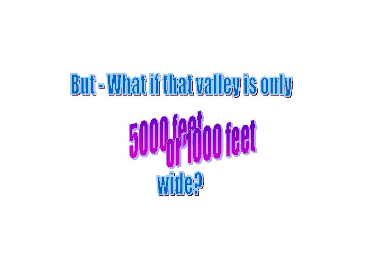
Edge effects Valley 1000’ wide Valley g=-3. 12 mg g=-4. 25 mg 5000’ The 3. 12 milligal anomaly implies a valley depth of only 406 feet. The 4. 25 milligal anomaly implies 550 feet bedrock depth. We have errors of 32% and 8. 3% in these two cases.

Topographic effects g. B may seem like a pretty unrealistic approximation of the topographic surface. It is. You had to scrape off all mountain tops above the observation elevation and fill in all the valleys when you made the plate correction. See figure 6. 3

- obviously we’re not through yet. We now have to scrape out those valleys put those hills back and compute their influence on gt …. i. e. we have to compensate for the effect of topography on the plate.

But back to the problem with the topographic surface. What is the effect of the topography on the observed gravity.

We estimate the effect of topography by approximating topographic features as ring-sectors whose thickness (z) equals the average elevation of topographic features within them.

Ri = inner radius of the ring Ro = outer radius of the ring z = thickness of the ring (average elevation of the topographic features inside the sector of interest) For a derivation, see Burger et al (2006) Also see Keary, Brooks and Hill (p 135) where constants are incorporated to simplify the computation-

The topographic effect gt is always negative. Again, this may seem like a crude approximation of actual topography. But topographic compensation is a laborious process and if done in detail the estimate is fairly accurate. We can increase the detail of our computation depending on the accuracy needed in a given application. Now that digital elevation data are available, we can actually let the computer do a very detailed computation using each digital elevation pixel. We’ll discuss methods used to compute the topographic effect more in the next lecture. The last term we will look at incorporates the effects of tide and instrument drift.

Tide and instrument drift We are used to thinking in terms of ocean tides. The ocean surface rises and falls under the influence of the combined gravitational attraction of the sun and moon. The solid earth also deforms under the influence in response to the differential pull of the sun and the moon. The change in surface elevation in addition to their gravitational pull on the gravimeter spring can be significant and these tidal effects must be incorporated into our estimate of theoretical gravity. Berger (1992)

The gravimeter is just a mechanical system. Its parts - while simple - change over time. The spring for example subjected to the constant tug of gravity will experience permanent changes in length over time. These changes fall under the heading of instrument drift. Berger (1992)

In general the influence of tide and drift on theoretical gravity is estimated by direct and repeated measurement of gravitational acceleration at the same place, over and over again, throughout the day. Usually during a survey a base station is reoccupied every couple hours or so during the day’s survey. The “drift curve” is constructed from these measurements and measurements of acceleration made at other stations are corrected relative to the drift curve.

Gravity observations M i l l i g a l s 4 3 2 1 8 Base 9 10 11 S 2 Base TIME (am) Is the acceleration of gravity measured at 9 am the same as that measured at the base station an hour earlier?

Drift Curve M i l l i g a l s 4 +1 m. G Tide & Drift Curve 3 2 -1 m. G 1 8 Base 9 10 S 1 S 2 TIME (am) 11 Base

In this example, the acceleration at station 1 (S 1) is 1 milligal less than that at the base station not the same. At station 2, the acceleration is only 1 milligal greater - not 3 milligals greater. M i l l i g a l s 4 +1 m. G 3 Tide and Drift Curve 2 -1 m. G 1 8 Base 9 S 1 TIME 10 S 2 11 Base

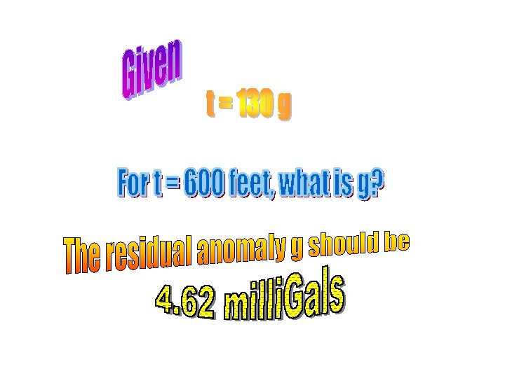
In the next computer lab (October 25 th) be prepared to ask questions about problems 6. 1 through 6. 3 handed out to you today. Also bring any questions you might have about Stewart’s paper to lab and concentrate on developing an understanding of how the gravitational acceleration of an infinite plate, whose thickness is equal to that of the glacial drift, can be used to estimate thickness of the drift. Realize that the use of the infinite plate to estimate drift thickness assumes that the drift valleys are much wider than they are thick. If that is so then the relationship t = 130 g provides an estimate of drift thickness.

density contrast t drift thickness If the valley width is much greater than its thickness, then the gravitational acceleration due to the drift is proportional to its thickness

As we conclude the day - do you have any questions about the model we’ve proposed to explain the gravitational acceleration at an arbitrary point on the surface of our theoretical (but geologically unrealistic) earth?

As geologists we expect there will be considerable subsurface density contrast associated, for example, with structure - or stratigraphy, drift thickness, caves, trenchs … In preparing our gravity data, we start by computing theoretical gravity but usually find that theoretical gravity we compute at a given latitude and elevation does not equal the observed gravity at that location.

We have an anomaly - And therein lies the geology.