Environmental and Exploration Geophysics I Gravity Methods VI

Environmental and Exploration Geophysics I Gravity Methods (VI) the terrain correction and the residual tom. h. wilson tom. wilson@mail. wvu. edu Department of Geology and Geography West Virginia University Morgantown, WV Tom Wilson, Department of Geology and Geography

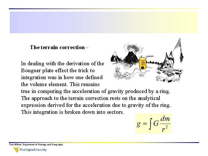
The terrain correction In dealing with the derivation of the Bouguer plate effect the trick to integration was in how one defined the volume element. This remains true in computing the acceleration of gravity produced by a ring. The approach to the terrain correction rests on the analytical expression derived for the acceleration due to gravity of the ring. This integration is broken down into sectors. Tom Wilson, Department of Geology and Geography

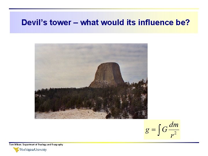
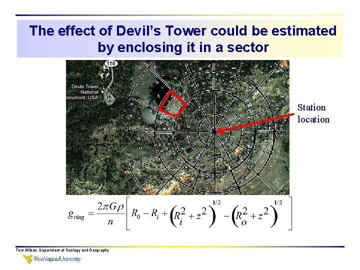
Devil’s tower – what would its influence be? Tom Wilson, Department of Geology and Geography

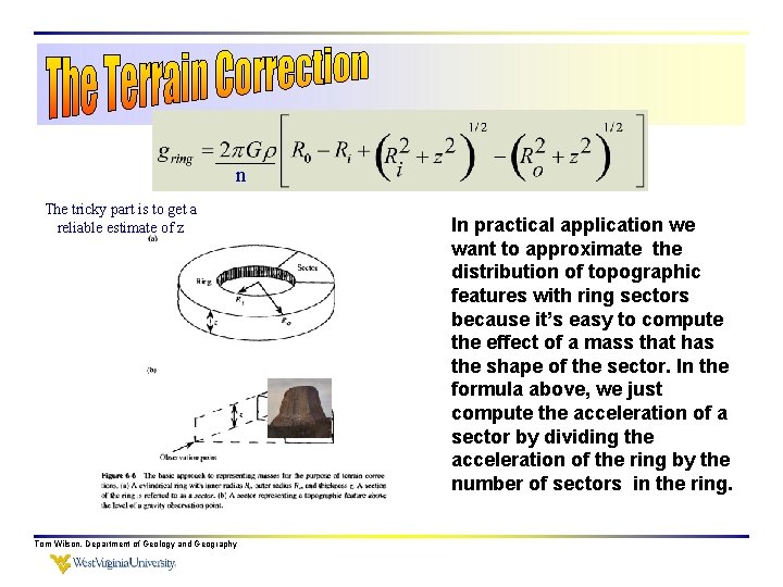
n The tricky part is to get a reliable estimate of z Tom Wilson, Department of Geology and Geography In practical application we want to approximate the distribution of topographic features with ring sectors because it’s easy to compute the effect of a mass that has the shape of the sector. In the formula above, we just compute the acceleration of a sector by dividing the acceleration of the ring by the number of sectors in the ring.

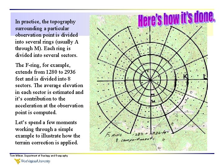
In practice, the topography surrounding a particular observation point is divided into several rings (usually A through M). Each ring is divided into several sectors. The F-ring, for example, extends from 1280 to 2936 feet and is divided into 8 sectors. The average elevation in each sector is estimated and it’s contribution to the acceleration at the observation point is computed. Let’s spend a few moments working through a simple example to illustrate how the terrain correction is applied. Tom Wilson, Department of Geology and Geography

The effect of Devil’s Tower could be estimated by enclosing it in a sector Station location Tom Wilson, Department of Geology and Geography

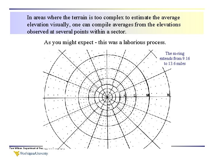
In areas where the terrain is too complex to estimate the average elevation visually, one can compile averages from the elevations observed at several points within a sector. As you might expect - this was a laborious process. The m-ring extends from 9. 16 to 13. 6 miles Tom Wilson, Department of Geology and Geography

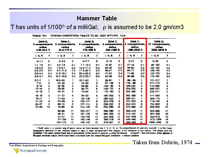
Hammer Table T has units of 1/100 th of a milli. Gal; is assumed to be 2. 0 gm/cm 3 Tom Wilson, Department of Geology and Geography Taken from Dobrin, 1974

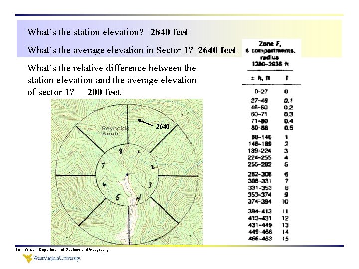
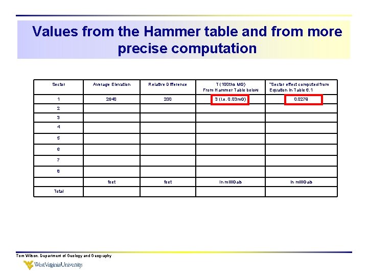
What’s the station elevation? 2840 feet What’s the average elevation in Sector 1? 2640 feet What’s the relative difference between the station elevation and the average elevation of sector 1? 200 feet 2640 Tom Wilson, Department of Geology and Geography

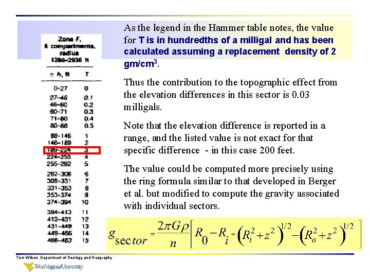
As the legend in the Hammer table notes, the value for T is in hundredths of a milligal and has been calculated assuming a replacement density of 2 gm/cm 3. Thus the contribution to the topographic effect from the elevation differences in this sector is 0. 03 milligals. Note that the elevation difference is reported in a range, and the listed value is not exact for that specific difference - in this case 200 feet. The value could be computed more precisely using the ring formula similar to that developed in Berger et al. but modified to compute the gravity associated with individual sectors. Tom Wilson, Department of Geology and Geography

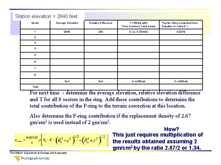
Station elevation = 2840 feet Sector Average Elevation Relative Difference T (100 ths MG) From Hammer Table below 1 2640 200 3 (i. e. 0. 03 m. G) 2640 2 200 *Sector effect computed from Equation in Table 6. 1 0. 0279 3 (0. 03 m. G) 0. 0279 m. G 3 4 5 6 7 8 feet In milli. Gals Total For next time - determine the average elevation, relative elevation difference and T for all 8 sectors in the ring. Add these contributions to determine the total contribution of the F-ring to the terrain correction at this location. Also determine the F-ring contribution if the replacement density of 2. 67 gm/cm 3 is used instead of 2 gm/cm 3. How? This just requires multiplication of the results obtained assuming 2 gm/cm 3 by the ratio 2. 67/2 or 1. 34. Tom Wilson, Department of Geology and Geography

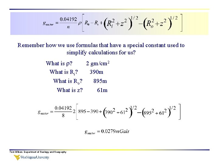
Remember how we use formulas that have a special constant used to simplify calculations for us? What is ? 2 gm/cm 2 What is Ri? 390 m What is Ro? 895 m What is z? Tom Wilson, Department of Geology and Geography 61 m

Values from the Hammer table and from more precise computation Sector Average Elevation Relative Difference T (100 ths MG) From Hammer Table below *Sector effect computed from Equation in Table 6. 1 1 2640 200 3 (i. e. 0. 03 m. G) 0. 0279 feet In milli. Gals 2 3 4 5 6 7 8 Total Tom Wilson, Department of Geology and Geography

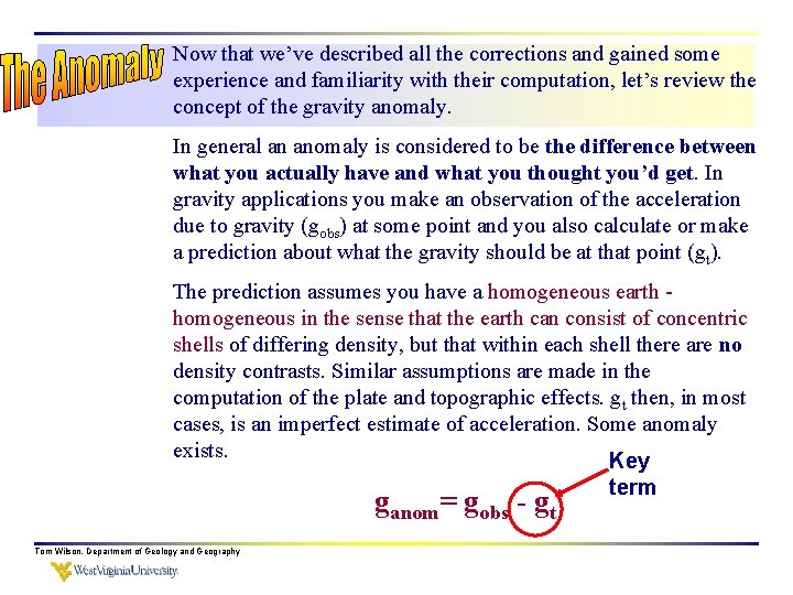
Now that we’ve described all the corrections and gained some experience and familiarity with their computation, let’s review the concept of the gravity anomaly. In general an anomaly is considered to be the difference between what you actually have and what you thought you’d get. In gravity applications you make an observation of the acceleration due to gravity (gobs) at some point and you also calculate or make a prediction about what the gravity should be at that point (gt). The prediction assumes you have a homogeneous earth homogeneous in the sense that the earth can consist of concentric shells of differing density, but that within each shell there are no density contrasts. Similar assumptions are made in the computation of the plate and topographic effects. gt then, in most cases, is an imperfect estimate of acceleration. Some anomaly exists. Key ganom= gobs - gt Tom Wilson, Department of Geology and Geography term

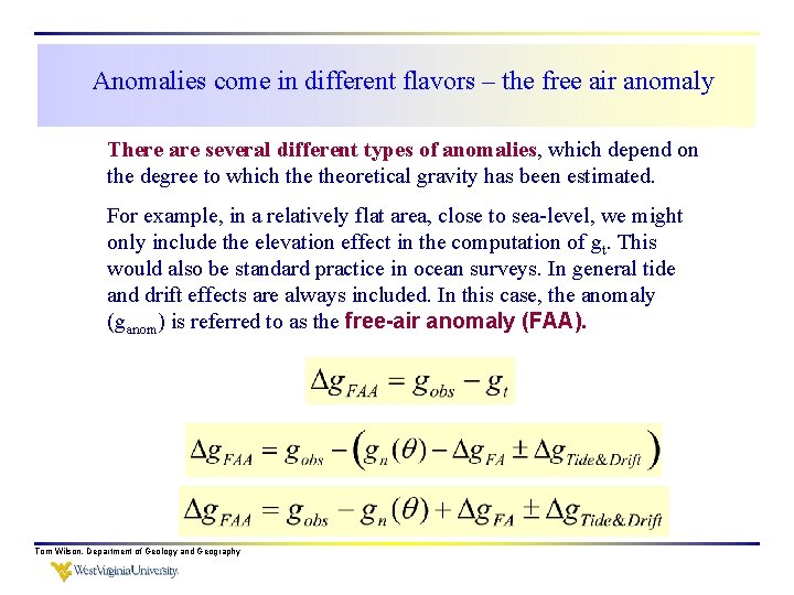
Anomalies come in different flavors – the free air anomaly There are several different types of anomalies, which depend on the degree to which theoretical gravity has been estimated. For example, in a relatively flat area, close to sea-level, we might only include the elevation effect in the computation of gt. This would also be standard practice in ocean surveys. In general tide and drift effects are always included. In this case, the anomaly (ganom) is referred to as the free-air anomaly (FAA). Tom Wilson, Department of Geology and Geography

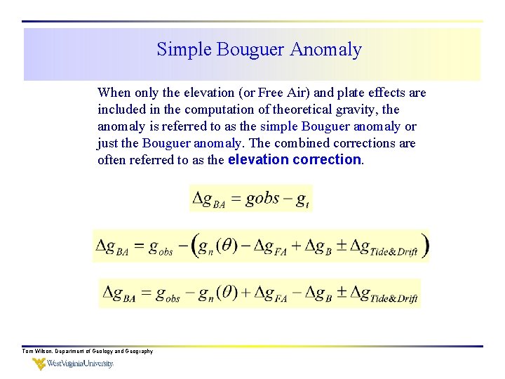
Simple Bouguer Anomaly When only the elevation (or Free Air) and plate effects are included in the computation of theoretical gravity, the anomaly is referred to as the simple Bouguer anomaly or just the Bouguer anomaly. The combined corrections are often referred to as the elevation correction. Tom Wilson, Department of Geology and Geography

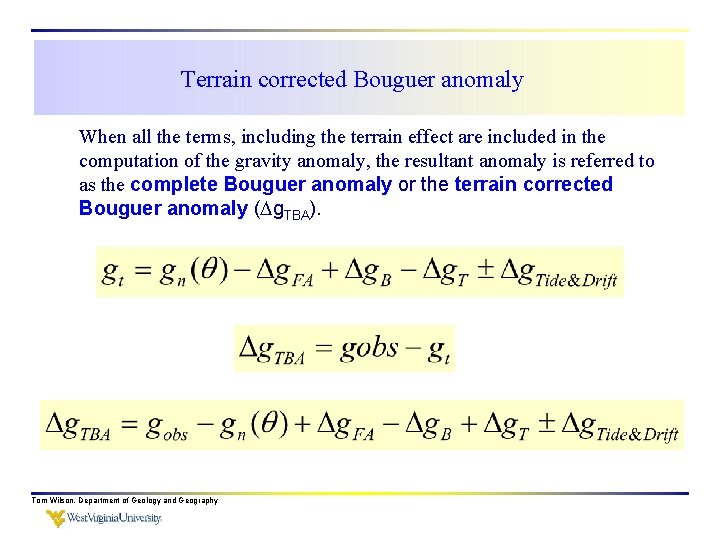
Terrain corrected Bouguer anomaly When all the terms, including the terrain effect are included in the computation of the gravity anomaly, the resultant anomaly is referred to as the complete Bouguer anomaly or the terrain corrected Bouguer anomaly ( g. TBA). Tom Wilson, Department of Geology and Geography

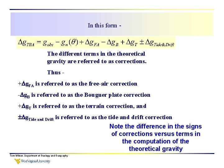
In this form - The different terms in theoretical gravity are referred to as corrections. Thus + g. FA is referred to as the free-air correction - g. B is referred to as the Bouguer plate correction + g. T is referred to as the terrain correction, and g. Tide and Drift is referred to as the tide and drift correction Note the difference in the signs of corrections versus terms in the computation of theoretical gravity Tom Wilson, Department of Geology and Geography

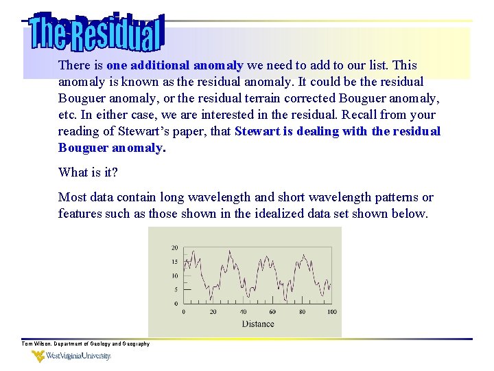
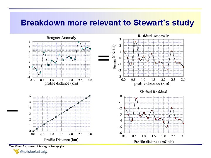
There is one additional anomaly we need to add to our list. This anomaly is known as the residual anomaly. It could be the residual Bouguer anomaly, or the residual terrain corrected Bouguer anomaly, etc. In either case, we are interested in the residual. Recall from your reading of Stewart’s paper, that Stewart is dealing with the residual Bouguer anomaly. What is it? Most data contain long wavelength and short wavelength patterns or features such as those shown in the idealized data set shown below. Tom Wilson, Department of Geology and Geography

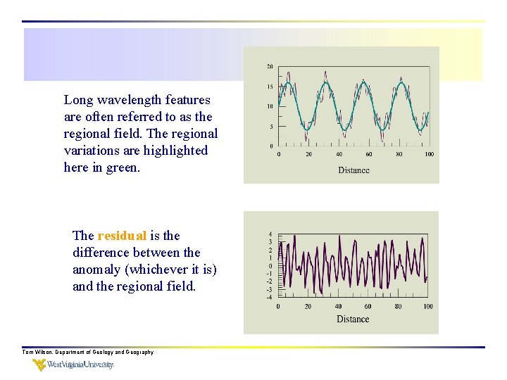
Long wavelength features are often referred to as the regional field. The regional variations are highlighted here in green. The residual is the difference between the anomaly (whichever it is) and the regional field. Tom Wilson, Department of Geology and Geography

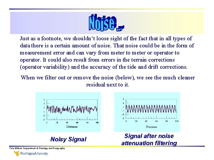
Just as a footnote, we shouldn’t loose sight of the fact that in all types of data there is a certain amount of noise. That noise could be in the form of measurement error and can vary from meter to meter or operator to operator. It could also result from errors in the terrain corrections (operator variability) and the accuracy of the tide and drift corrections. When we filter out or remove the noise (below), we see the much cleaner residual next to it. Noisy Signal Tom Wilson, Department of Geology and Geography Signal after noise attenuation filtering

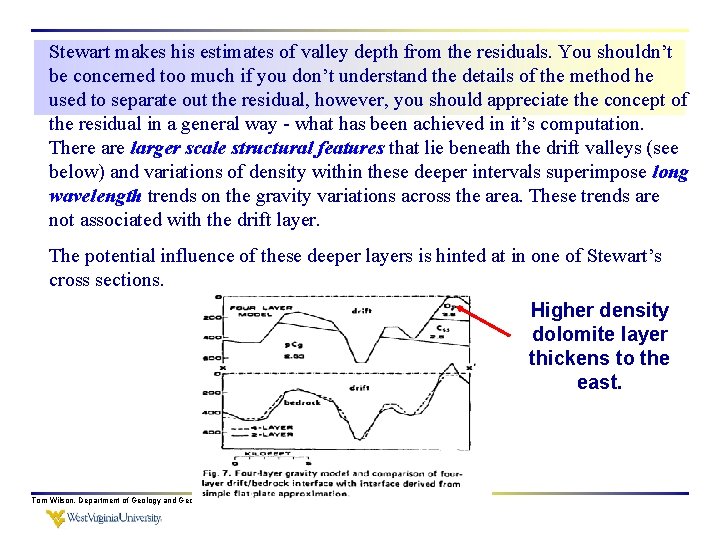
Stewart makes his estimates of valley depth from the residuals. You shouldn’t be concerned too much if you don’t understand the details of the method he used to separate out the residual, however, you should appreciate the concept of the residual in a general way - what has been achieved in it’s computation. There are larger scale structural features that lie beneath the drift valleys (see below) and variations of density within these deeper intervals superimpose long wavelength trends on the gravity variations across the area. These trends are not associated with the drift layer. The potential influence of these deeper layers is hinted at in one of Stewart’s cross sections. Higher density dolomite layer thickens to the east. Tom Wilson, Department of Geology and Geography

Breakdown more relevant to Stewart’s study Tom Wilson, Department of Geology and Geography

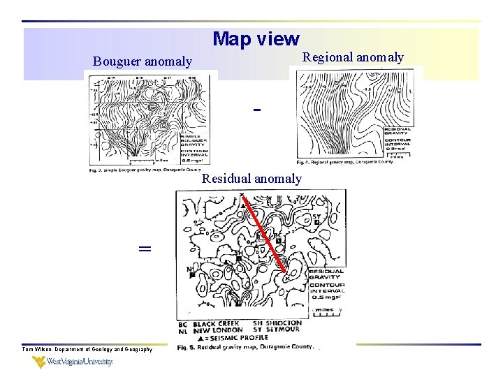
Map view Bouguer anomaly Residual anomaly = Tom Wilson, Department of Geology and Geography Regional anomaly

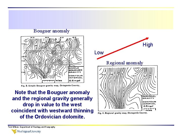
Bouguer anomaly High Low Regional anomaly Note that the Bouguer anomaly and the regional gravity generally drop in value to the west coincident with westward thinning of the Ordovician dolomite. Tom Wilson, Department of Geology and Geography

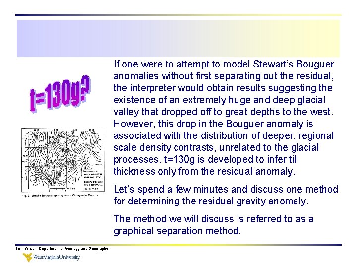
If one were to attempt to model Stewart’s Bouguer anomalies without first separating out the residual, the interpreter would obtain results suggesting the existence of an extremely huge and deep glacial valley that dropped off to great depths to the west. However, this drop in the Bouguer anomaly is associated with the distribution of deeper, regional scale density contrasts, unrelated to the glacial processes. t=130 g is developed to infer till thickness only from the residual anomaly. Let’s spend a few minutes and discuss one method for determining the residual gravity anomaly. The method we will discuss is referred to as a graphical separation method. Tom Wilson, Department of Geology and Geography

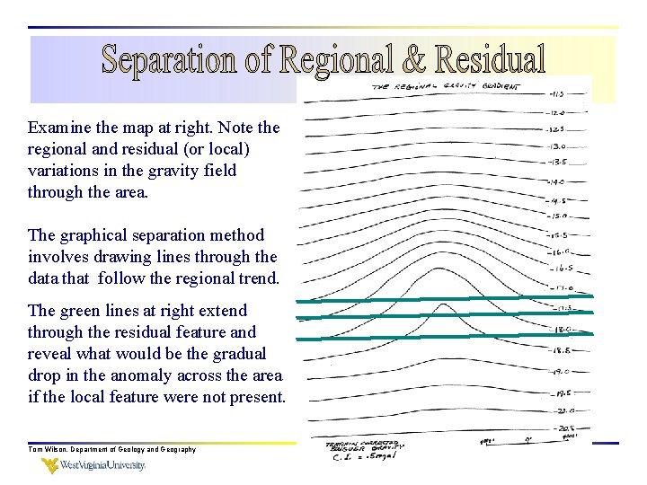
Examine the map at right. Note the regional and residual (or local) variations in the gravity field through the area. The graphical separation method involves drawing lines through the data that follow the regional trend. The green lines at right extend through the residual feature and reveal what would be the gradual drop in the anomaly across the area if the local feature were not present. Tom Wilson, Department of Geology and Geography

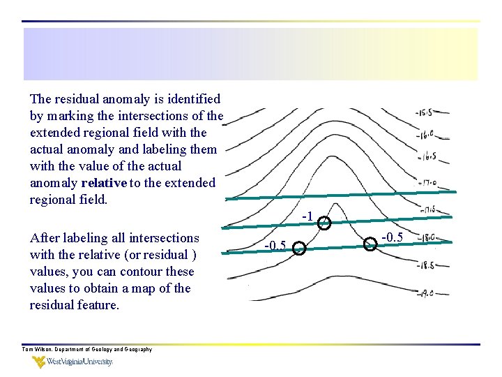
The residual anomaly is identified by marking the intersections of the extended regional field with the actual anomaly and labeling them with the value of the actual anomaly relative to the extended regional field. -1 After labeling all intersections with the relative (or residual ) values, you can contour these values to obtain a map of the residual feature. Tom Wilson, Department of Geology and Geography -0. 5

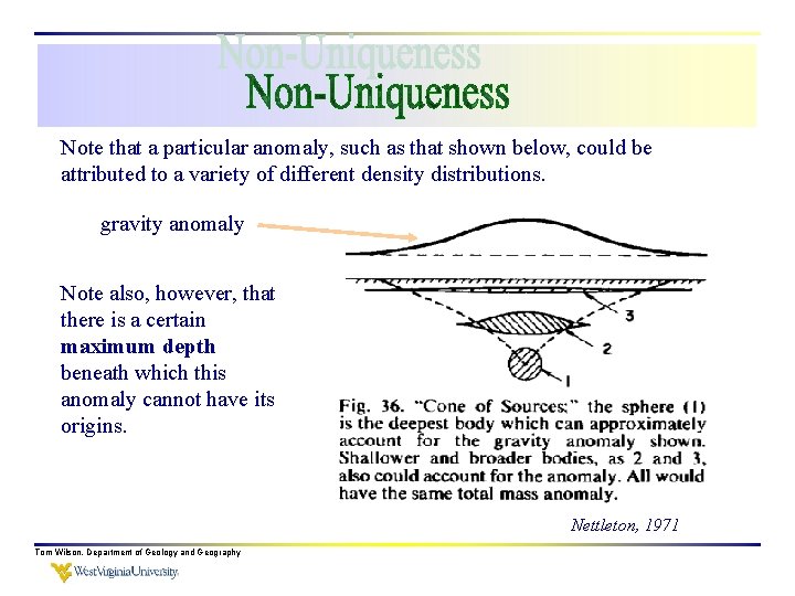
Note that a particular anomaly, such as that shown below, could be attributed to a variety of different density distributions. gravity anomaly Note also, however, that there is a certain maximum depth beneath which this anomaly cannot have its origins. Nettleton, 1971 Tom Wilson, Department of Geology and Geography

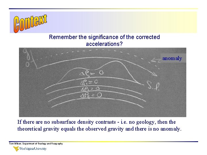
Remember the significance of the corrected accelerations? anomaly If there are no subsurface density contrasts - i. e. no geology, then theoretical gravity equals the observed gravity and there is no anomaly. Tom Wilson, Department of Geology and Geography

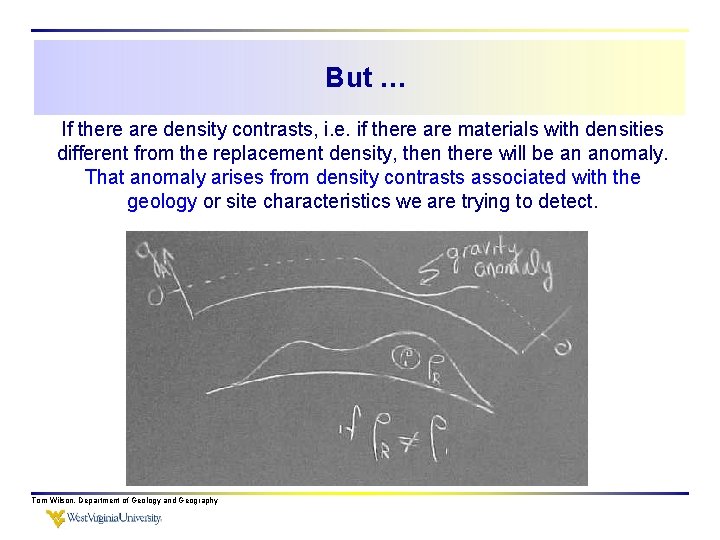
But … If there are density contrasts, i. e. if there are materials with densities different from the replacement density, then there will be an anomaly. That anomaly arises from density contrasts associated with the geology or site characteristics we are trying to detect. Tom Wilson, Department of Geology and Geography

Items on the list …. • Turn in your gravity paper summaries this Thursday, Nov. 5 th. • Gravity lab is due this Thursday. • Any final questions about the Gravity Lab? • Turn in tide and drift problem 6. 3 next Tuesday. • Start reading Chapter 7 – we will transition to Magnetic methods next Tuesday (and perhaps this Thursday). Tom Wilson, Department of Geology and Geography

Follow the standard reporting format. Include the following or similar subdivisions: Abstract: a brief description of what you did and the results you obtained (~200 words). Background: Provide some background on the data we’re analyzing. All of this would come from Stewart’s paper. Explain his approach and answer question 1 below in this section to illustrate his approach. Results: Describe how you tested the model proposed by Stewart along XX’. Include answers to questions 2 through 4 below in this discussion. Conclusions: Summarize the highlights of results obtained in the forgoing modeling process. Tom Wilson, Department of Geology and Geography

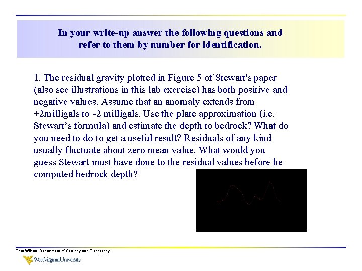
In your write-up answer the following questions and refer to them by number for identification. 1. The residual gravity plotted in Figure 5 of Stewart's paper (also see illustrations in this lab exercise) has both positive and negative values. Assume that an anomaly extends from +2 milligals to -2 milligals. Use the plate approximation (i. e. Stewart’s formula) and estimate the depth to bedrock? What do you need to do to get a useful result? Residuals of any kind usually fluctuate about zero mean value. What would you guess Stewart must have done to the residual values before he computed bedrock depth? Tom Wilson, Department of Geology and Geography

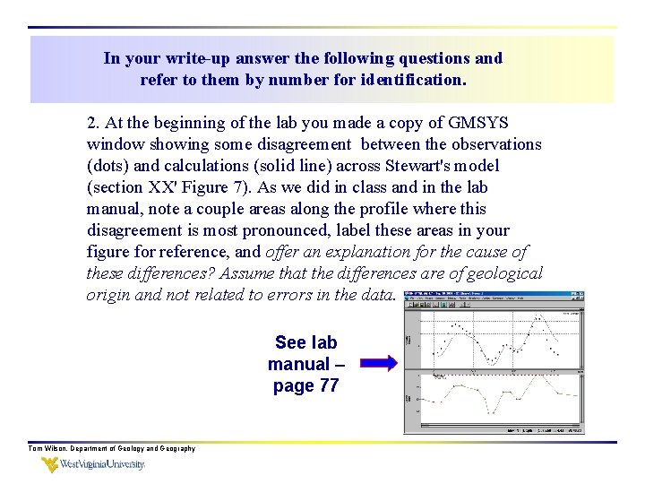
In your write-up answer the following questions and refer to them by number for identification. 2. At the beginning of the lab you made a copy of GMSYS window showing some disagreement between the observations (dots) and calculations (solid line) across Stewart's model (section XX' Figure 7). As we did in class and in the lab manual, note a couple areas along the profile where this disagreement is most pronounced, label these areas in your figure for reference, and offer an explanation for the cause of these differences? Assume that the differences are of geological origin and not related to errors in the data. See lab manual – page 77 Tom Wilson, Department of Geology and Geography

In your write-up answer the following questions and refer to them by number for identification. 3. With a combination of inversion and manual adjustments of points defining the till/bedrock interface, you were able to eliminate the significant differences between observed and calculated gravity. Although you have good agreement between the observations and calculations, do you think the model could still be in error? How does the model oversimplify the geology? Consider the influence of edge effects in and out of the section (using 2 ¾ modeling option) as well as those along the section. These edge effects were illustrated and computed on several occasions in class. Just repeat those arguments and show your own calculations. Also refer to Stewart’s gravity anomaly map. Tom Wilson, Department of Geology and Geography

In your write-up answer the following questions and refer to them by number for identification. 4. After inversion, does the plate approximation (expressed in Stewart's formula t = 130 g) provide reliable estimates of bedrock depth in this area? Provide two examples taken from the data and model you developed in lab. It is important to separate the use of the equation t = 130 g from the inverse models you’ve developed using GMSYS. t=130 g makes simplifying assumptions and allows you to make quick judgments about the location of the glacial valleys and their depths. GMSYS does a more precise computation of valley depth, but also includes some underlying assumptions. Tom Wilson, Department of Geology and Geography

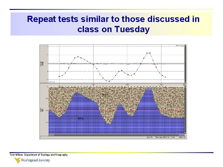
Repeat tests similar to those discussed in class on Tuesday Tom Wilson, Department of Geology and Geography

Include responses to the above questions and observations in your discussion of Stewart's paper. Use figures you've generated in GMSYS to illustrate your point. All figures should be numbered, labeled and captioned. Tom Wilson, Department of Geology and Geography

See you Tuesday … • Hand in problems 6. 1 – 6. 3 • Magnetic papers are in the mail room. • Start reading Chapter 7 – we will transition to Magnetic methods next Tuesday (and perhaps this Thursday). • Gravity lab is due next Tuesday. Tom Wilson, Department of Geology and Geography