ENGG 2013 Unit 24 Linear DE and Applications

ENGG 2013 Unit 24 Linear DE and Applications Apr, 2011.

Outline • Method of separating variable • Method of integrating factor • System of linear and first-order differential equations – Graphical method using phase plane kshum 2

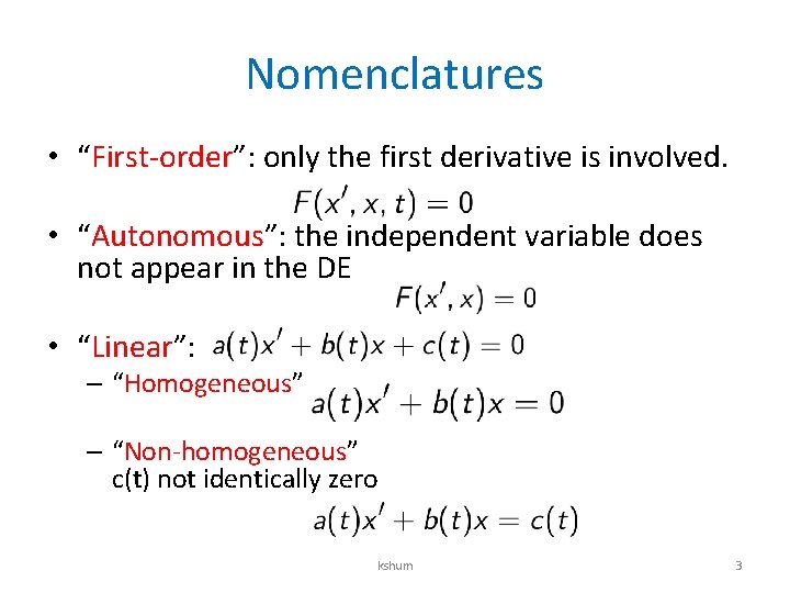
Nomenclatures • “First-order”: only the first derivative is involved. • “Autonomous”: the independent variable does not appear in the DE • “Linear”: – “Homogeneous” – “Non-homogeneous” c(t) not identically zero kshum 3

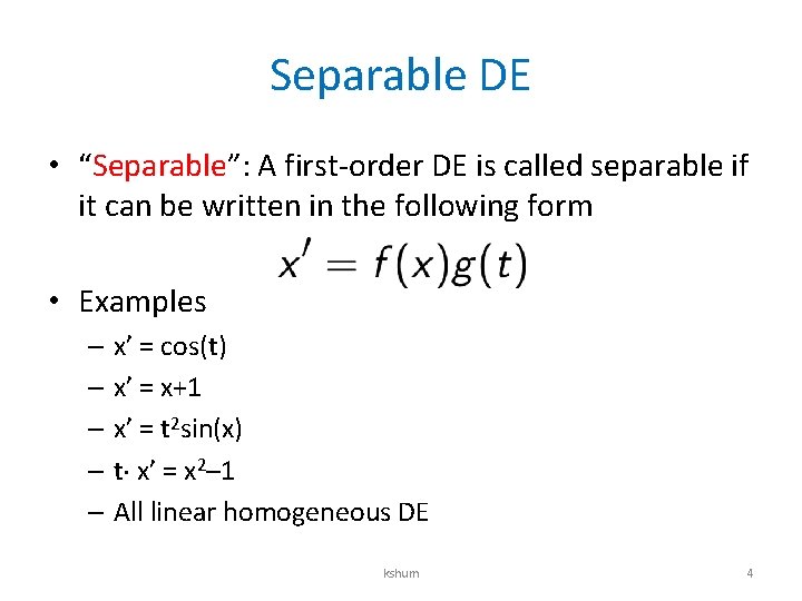
Separable DE • “Separable”: A first-order DE is called separable if it can be written in the following form • Examples – x’ = cos(t) – x’ = x+1 – x’ = t 2 sin(x) – t x’ = x 2– 1 – All linear homogeneous DE kshum 4

SEPARABLE DE AND METHOD OF SEPARATING VARIABLES kshum 5

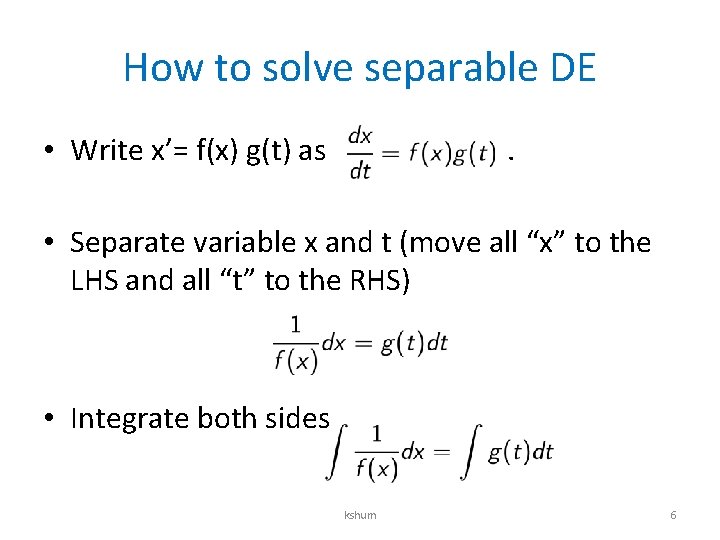
How to solve separable DE • Write x’= f(x) g(t) as . • Separate variable x and t (move all “x” to the LHS and all “t” to the RHS) • Integrate both sides kshum 6

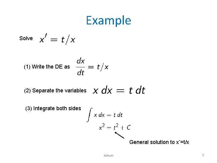
Example Solve (1) Write the DE as (2) Separate the variables (3) Integrate both sides General solution to x’=t/x kshum 7

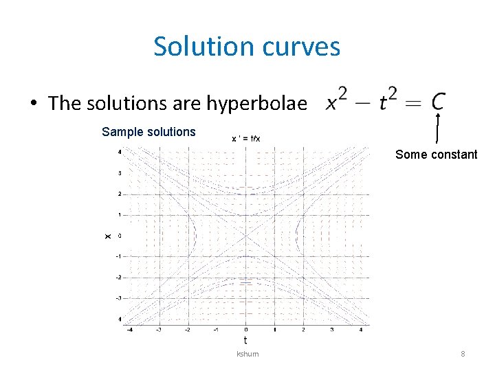
Solution curves • The solutions are hyperbolae Sample solutions Some constant kshum 8

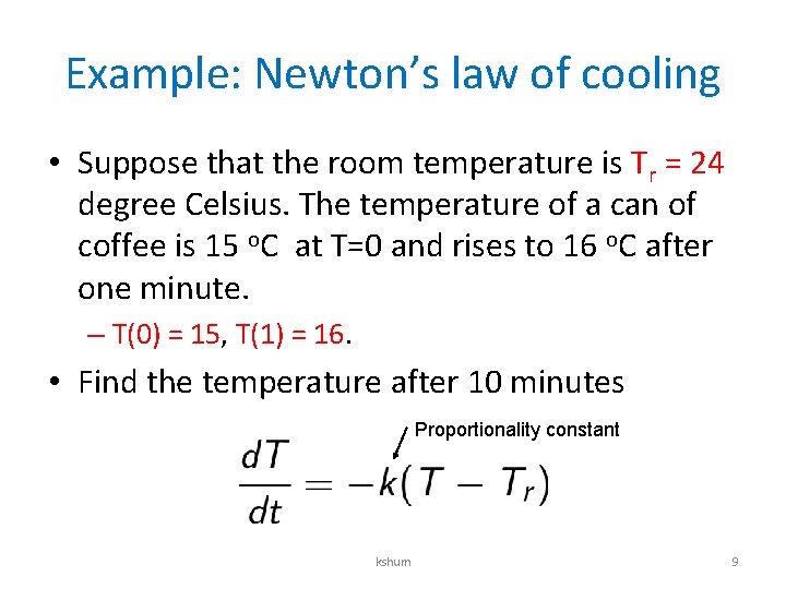
Example: Newton’s law of cooling • Suppose that the room temperature is Tr = 24 degree Celsius. The temperature of a can of coffee is 15 o. C at T=0 and rises to 16 o. C after one minute. – T(0) = 15, T(1) = 16. • Find the temperature after 10 minutes Proportionality constant kshum 9

LINEAR NON-HOMOGENEOUS DE METHOD OF INTEGRATING FACTOR kshum 10

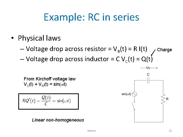
Example: RC in series • Physical laws – Voltage drop across resistor = VR(t) = R I(t) – Voltage drop across inductor = C VC(t) = Q(t) Charge From Kirchoff voltage law VC(t) + VR(t) = sin( t) Linear non-homogeneous kshum 11

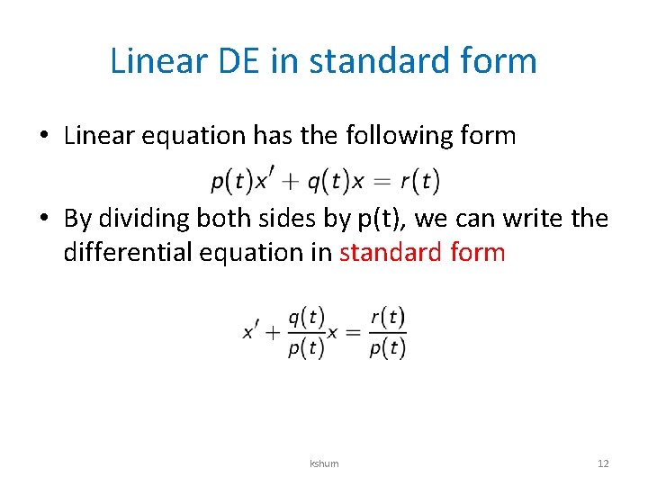
Linear DE in standard form • Linear equation has the following form • By dividing both sides by p(t), we can write the differential equation in standard form kshum 12

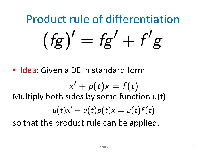
Product rule of differentiation • Idea: Given a DE in standard form Multiply both sides by some function u(t) so that the product rule can be applied. kshum 13

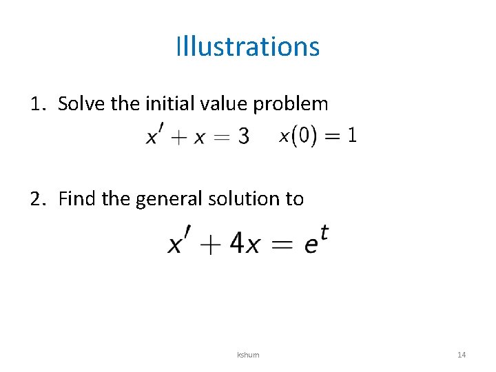
Illustrations 1. Solve the initial value problem 2. Find the general solution to kshum 14

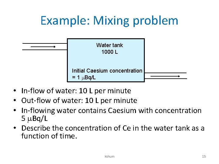
Example: Mixing problem Water tank 1000 L Initial Caesium concentration = 1 Bq/L • In-flow of water: 10 L per minute • Out-flow of water: 10 L per minute • In-flowing water contains Caesium with concentration 5 Bq/L • Describe the concentration of Ce in the water tank as a function of time. kshum 15

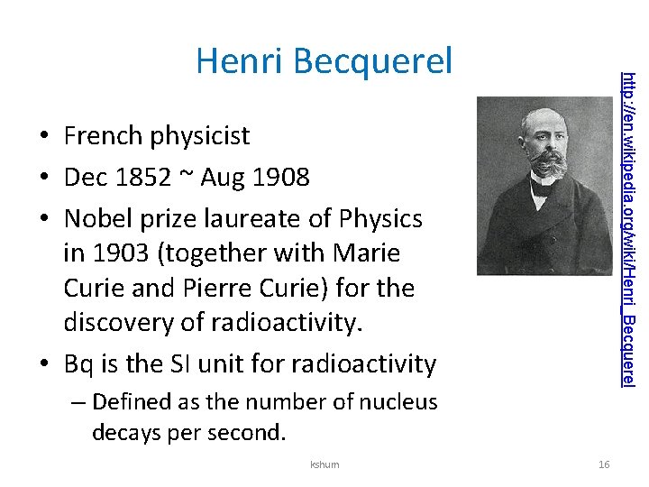
http: //en. wikipedia. org/wiki/Henri_Becquerel Henri Becquerel • French physicist • Dec 1852 ~ Aug 1908 • Nobel prize laureate of Physics in 1903 (together with Marie Curie and Pierre Curie) for the discovery of radioactivity. • Bq is the SI unit for radioactivity – Defined as the number of nucleus decays per second. kshum 16

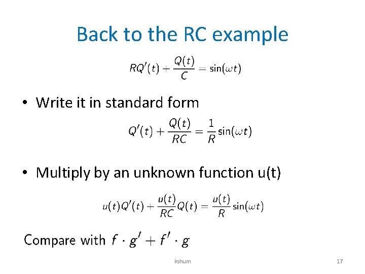
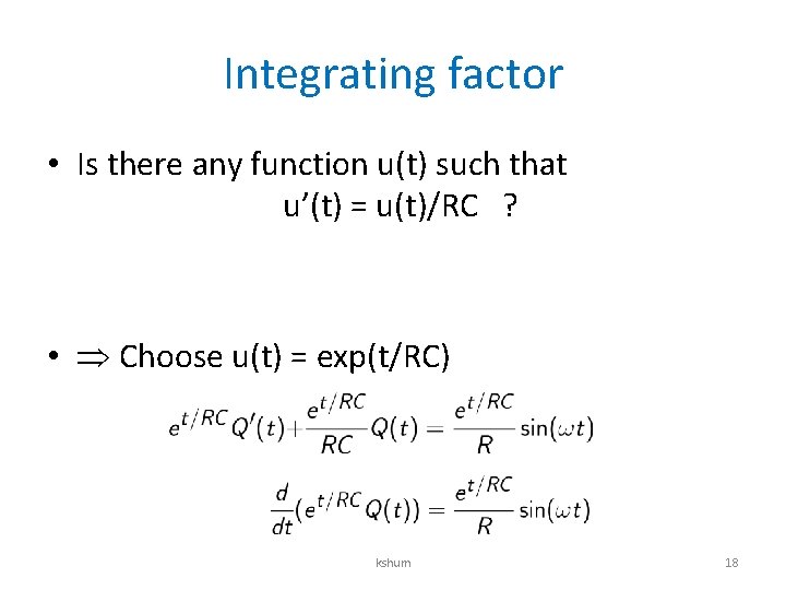
Back to the RC example • Write it in standard form • Multiply by an unknown function u(t) kshum 17

Integrating factor • Is there any function u(t) such that u’(t) = u(t)/RC ? • Choose u(t) = exp(t/RC) kshum 18

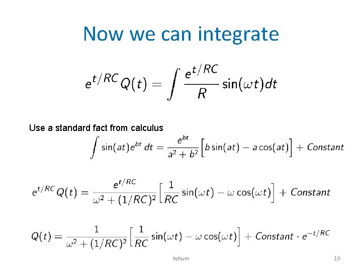
Now we can integrate Use a standard fact from calculus kshum 19

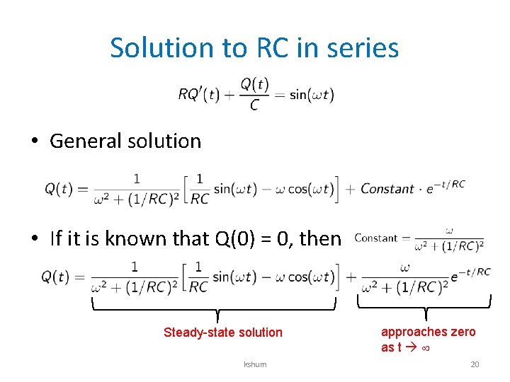
Solution to RC in series • General solution • If it is known that Q(0) = 0, then Steady-state solution kshum approaches zero as t 20

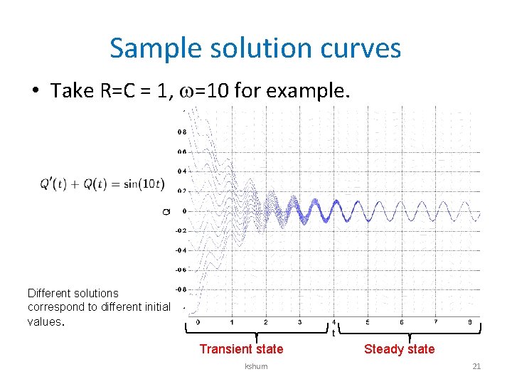
Sample solution curves • Take R=C = 1, =10 for example. Different solutions correspond to different initial values. Transient state kshum Steady state 21

SYSTEM OF DIFFERENTIAL EQUATIONS kshum 22

Interaction between components • If we have two or more objects, each and they interact with each other, we need a system of differential equations. • Metronomes synchronization – http: //www. youtube. com/watch? v=yysnk. Y 4 WHy. M • Double pendulum – http: //www. youtube. com/watch? v=p. YPRnx. S 6 u. Aw kshum 23

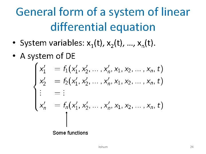
General form of a system of linear differential equation • System variables: x 1(t), x 2(t), …, xn(t). • A system of DE Some functions kshum 24

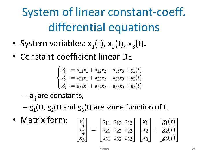
System of linear constant-coeff. differential equations • System variables: x 1(t), x 2(t), x 3(t). • Constant-coefficient linear DE – aij are constants, – g 1(t), g 2(t) and g 3(t) are some function of t. • Matrix form: kshum 25

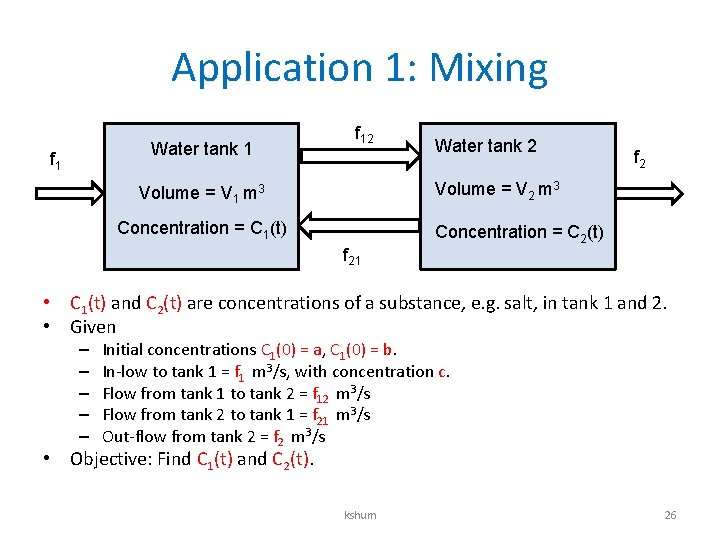
Application 1: Mixing Water tank 1 f 12 Water tank 2 f 2 Volume = V 2 m 3 Volume = V 1 m 3 Concentration = C 1(t) f 21 Concentration = C 2(t) • C 1(t) and C 2(t) are concentrations of a substance, e. g. salt, in tank 1 and 2. • Given – – – Initial concentrations C 1(0) = a, C 1(0) = b. In-low to tank 1 = f 1 m 3/s, with concentration c. Flow from tank 1 to tank 2 = f 12 m 3/s Flow from tank 2 to tank 1 = f 21 m 3/s Out-flow from tank 2 = f 2 m 3/s • Objective: Find C 1(t) and C 2(t). kshum 26

Modeling • • Consider a short time interval [t, t+ t] C 1 = C 1(t+ t)–C 1(t) = cf 1 t + f 21 C 2 t – f 12 C 1 t C 2 = C 2(t+ t)–C 2(t) = f 12 C 1 t – f 21 C 2 t – f 2 C 2 t Take t 0, we have C 1’ = – f 12 C 1 + f 21 C 2+ cf 1 C 2’ = f 12 C 1 – (f 21+ f 2) C 2 kshum 27

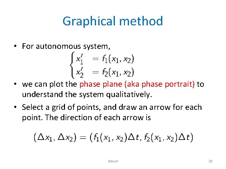
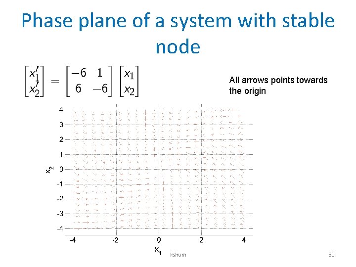
Graphical method • For autonomous system, • we can plot the phase plane (aka phase portrait) to understand the system qualitatively. • Select a grid of points, and draw an arrow for each point. The direction of each arrow is kshum 28

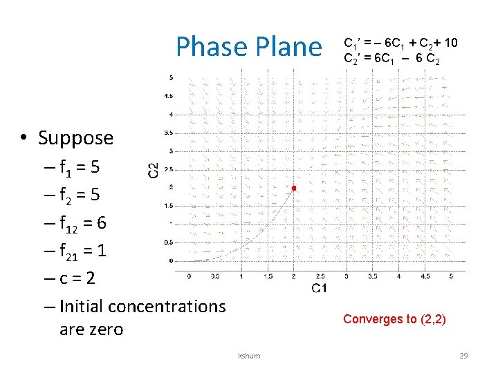
Phase Plane C 1’ = – 6 C 1 + C 2+ 10 C 2’ = 6 C 1 – 6 C 2 • Suppose – f 1 = 5 – f 2 = 5 – f 12 = 6 – f 21 = 1 –c=2 – Initial concentrations are zero Converges to (2, 2) kshum 29

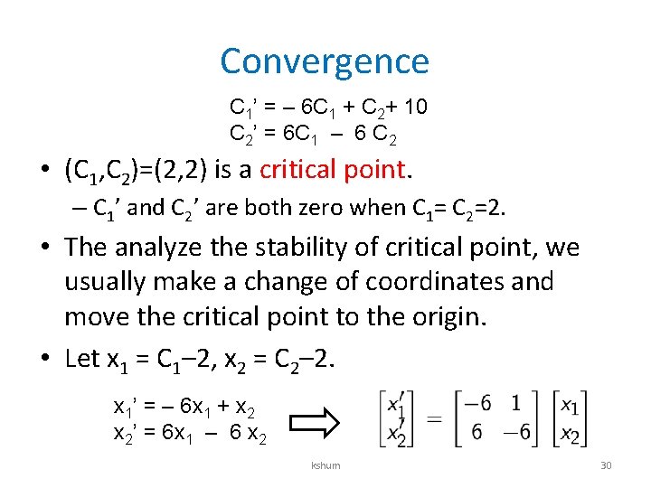
Convergence C 1’ = – 6 C 1 + C 2+ 10 C 2’ = 6 C 1 – 6 C 2 • (C 1, C 2)=(2, 2) is a critical point. – C 1’ and C 2’ are both zero when C 1= C 2=2. • The analyze the stability of critical point, we usually make a change of coordinates and move the critical point to the origin. • Let x 1 = C 1– 2, x 2 = C 2– 2. x 1’ = – 6 x 1 + x 2’ = 6 x 1 – 6 x 2 kshum 30

Phase plane of a system with stable node All arrows points towards the origin kshum 31

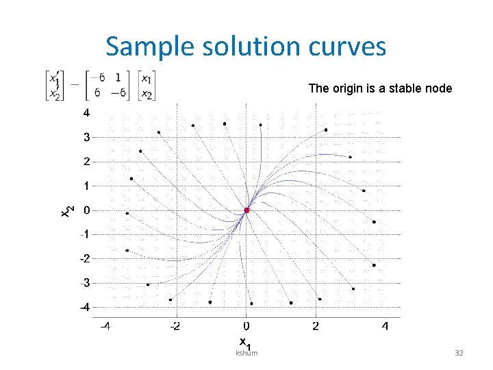
Sample solution curves The origin is a stable node kshum 32

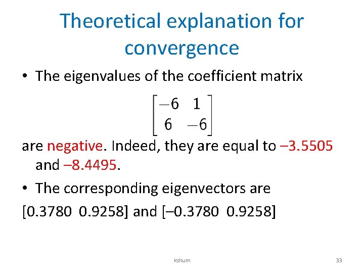
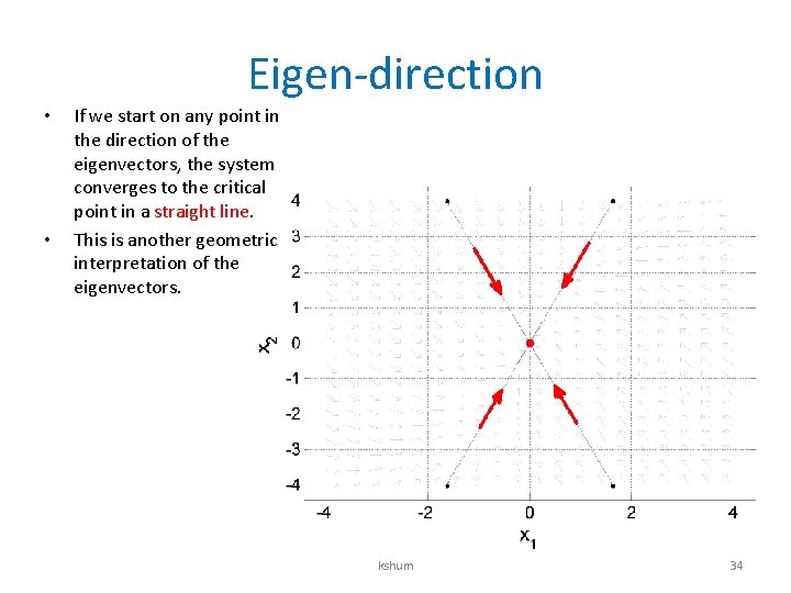
Theoretical explanation for convergence • The eigenvalues of the coefficient matrix are negative. Indeed, they are equal to – 3. 5505 and – 8. 4495. • The corresponding eigenvectors are [0. 3780 0. 9258] and [– 0. 3780 0. 9258] kshum 33

Eigen-direction • • If we start on any point in the direction of the eigenvectors, the system converges to the critical point in a straight line. This is another geometric interpretation of the eigenvectors. kshum 34

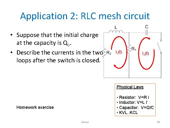
Application 2: RLC mesh circuit • Suppose that the initial charge at the capacity is Q 0. • Describe the currents in the two loops after the switch is closed. i 1(t) i 2(t) Physical Laws • Resistor: V=R i • Inductor: V=L i’ • Capacitor: V=Q/C • KVL, KCL Homework exercise kshum 35

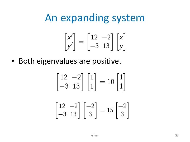
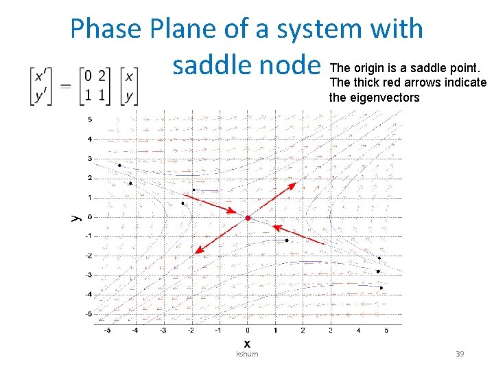
An expanding system • Both eigenvalues are positive. kshum 36

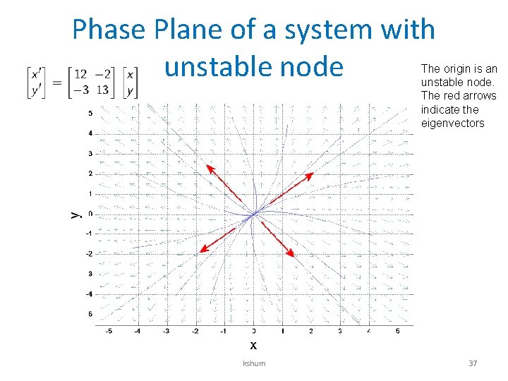
Phase Plane of a system with unstable node The origin is an unstable node. The red arrows indicate the eigenvectors kshum 37

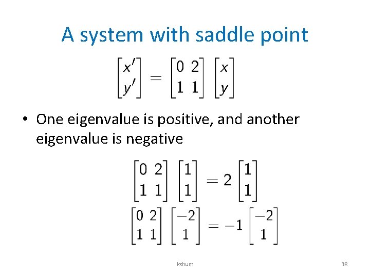
A system with saddle point • One eigenvalue is positive, and another eigenvalue is negative kshum 38

Phase Plane of a system with origin is a saddle point. saddle node The thick red arrows indicate the eigenvectors kshum 39

Conclusion The convergence and stability of a system of linear equations is intimately related to the signs of eigenvalues. kshum 40