EECS 583 Class 14 Modulo Scheduling Reloaded University

EECS 583 – Class 14 Modulo Scheduling Reloaded University of Michigan October 31, 2012

Announcements + Reading Material v Project proposals » Due Friday, Nov 2, 5 pm » 1 paragraph summary of what you plan to work on Ÿ Topic, approach, objective (performance, energy, code size) » 1 -2 references » Email to me&James, cc your group members v Today’s class reading » "Code Generation Schema for Modulo Scheduled Loops", B. Rau, M. Schlansker, and P. Tirumalai, MICRO-25, Dec. 1992. v Next reading – Last class before research stuff! » “Register Allocation and Spilling Via Graph Coloring, ” G. Chaitin, Proc. 1982 SIGPLAN Symposium on Compiler Construction, 1982. -1 -

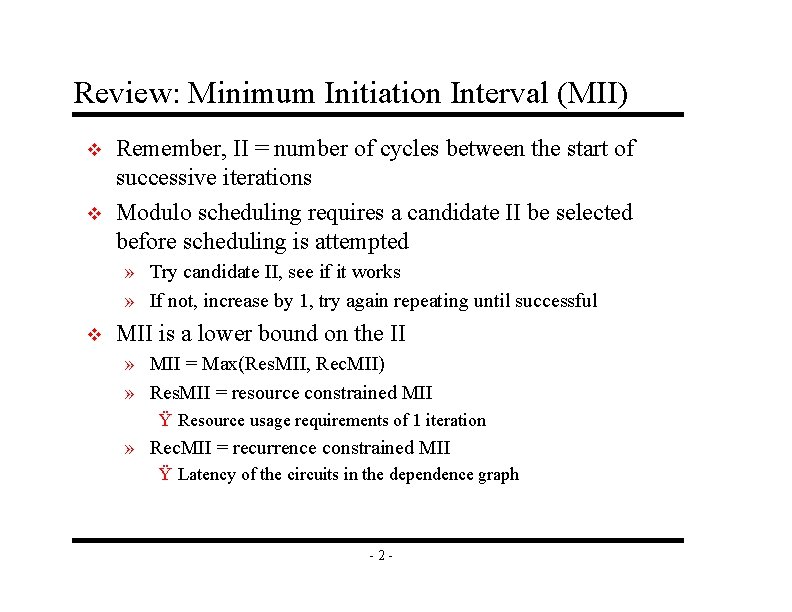
Review: Minimum Initiation Interval (MII) v v Remember, II = number of cycles between the start of successive iterations Modulo scheduling requires a candidate II be selected before scheduling is attempted » Try candidate II, see if it works » If not, increase by 1, try again repeating until successful v MII is a lower bound on the II » MII = Max(Res. MII, Rec. MII) » Res. MII = resource constrained MII Ÿ Resource usage requirements of 1 iteration » Rec. MII = recurrence constrained MII Ÿ Latency of the circuits in the dependence graph -2 -

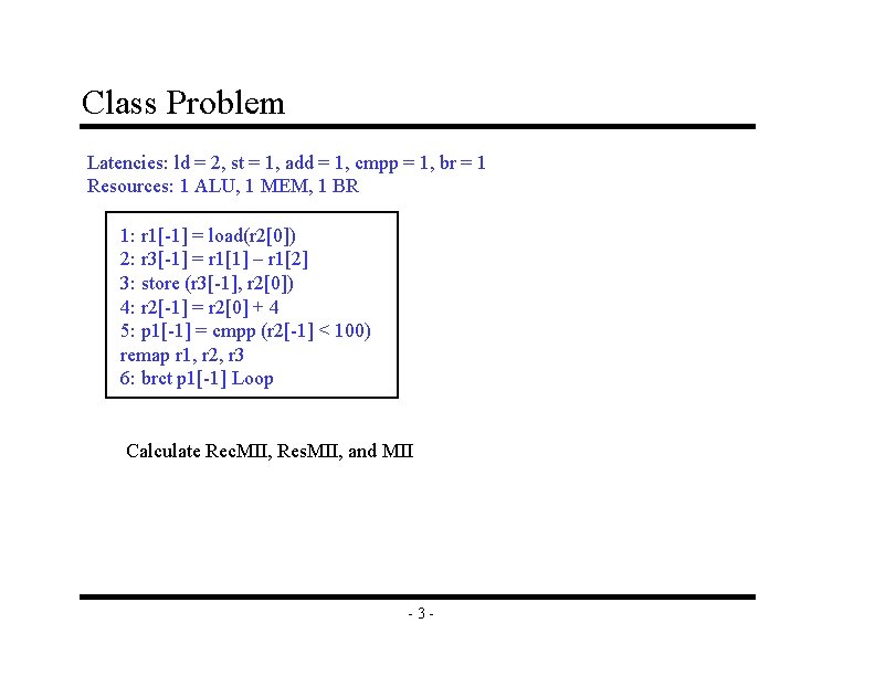
Class Problem Latencies: ld = 2, st = 1, add = 1, cmpp = 1, br = 1 Resources: 1 ALU, 1 MEM, 1 BR 1: r 1[-1] = load(r 2[0]) 2: r 3[-1] = r 1[1] – r 1[2] 3: store (r 3[-1], r 2[0]) 4: r 2[-1] = r 2[0] + 4 5: p 1[-1] = cmpp (r 2[-1] < 100) remap r 1, r 2, r 3 6: brct p 1[-1] Loop Calculate Rec. MII, Res. MII, and MII -3 -

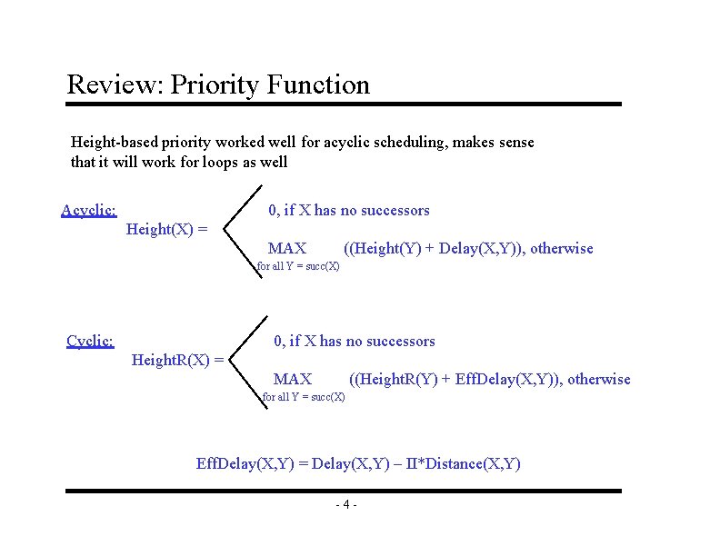
Review: Priority Function Height-based priority worked well for acyclic scheduling, makes sense that it will work for loops as well Acyclic: 0, if X has no successors Height(X) = MAX ((Height(Y) + Delay(X, Y)), otherwise for all Y = succ(X) Cyclic: 0, if X has no successors Height. R(X) = MAX ((Height. R(Y) + Eff. Delay(X, Y)), otherwise for all Y = succ(X) Eff. Delay(X, Y) = Delay(X, Y) – II*Distance(X, Y) -4 -

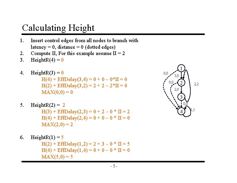
Calculating Height 1. 2. 3. 4. 5. 6. Insert control edges from all nodes to branch with latency = 0, distance = 0 (dotted edges) Compute II, For this example assume II = 2 Height. R(4) = 0 Height. R(3) = 0 H(4) + Eff. Delay(3, 4) = 0 + 0 – 0*II = 0 H(2) + Eff. Delay(3, 2) = 2 + 2 – 2*II = 0 MAX(0, 0) = 0 Height. R(2) = 2 H(3) + Eff. Delay(2, 3) = 0 + 2 – 0 * II = 2 H(4) + Eff. Delay(2, 4) = 0 + 0 – 0 * II = 0 MAX(2, 0) = 2 Height. R(1) = 5 H(2) + Eff. Delay(1, 2) = 2 + 3 – 0 * II = 5 H(4) + Eff. Delay(1, 4) = 0 + 0 – 0 * II = 0 MAX(5, 0) = 5 -5 - 1 0, 0 3, 0 2 0, 0 2, 2 2, 0 3 0, 0 4 1, 1

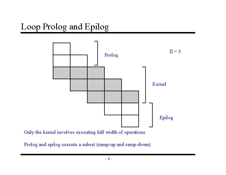
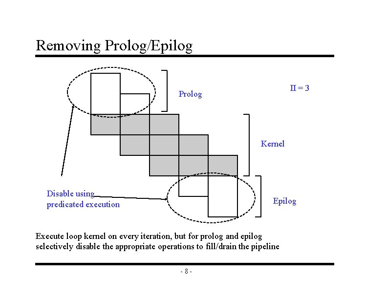
Loop Prolog and Epilog II = 3 Prolog Kernel Epilog Only the kernel involves executing full width of operations Prolog and epilog execute a subset (ramp-up and ramp-down) -6 -

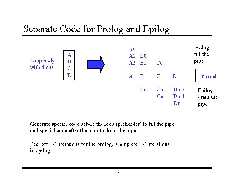
Separate Code for Prolog and Epilog Loop body with 4 ops A B C D Prolog fill the pipe A 0 A 1 B 0 A 2 B 1 C 0 A B C D Bn Cn-1 Cn Dn-2 Dn-1 Dn Generate special code before the loop (preheader) to fill the pipe and special code after the loop to drain the pipe. Peel off II-1 iterations for the prolog. Complete II-1 iterations in epilog -7 - Kernel Epilog drain the pipe

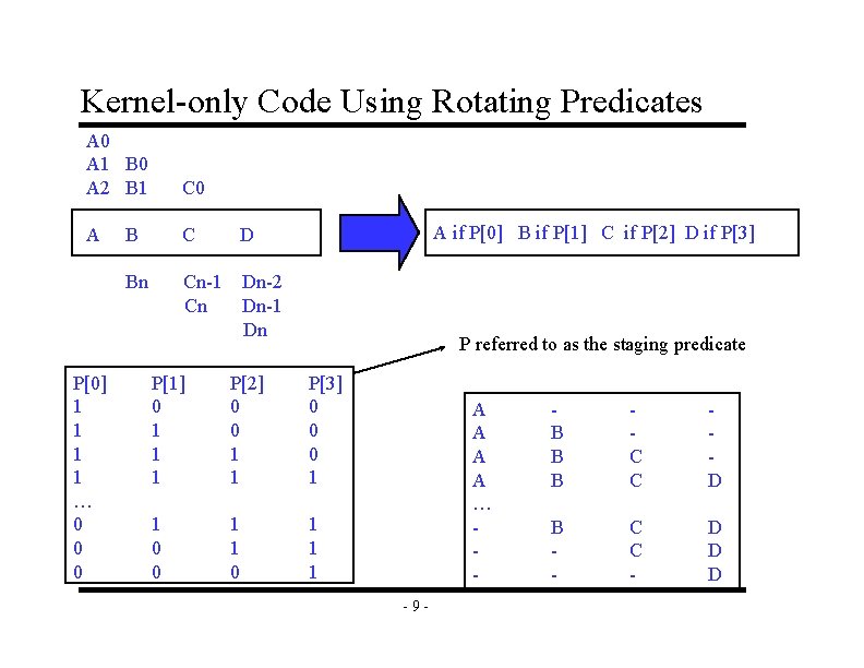
Removing Prolog/Epilog II = 3 Prolog Kernel Disable using predicated execution Epilog Execute loop kernel on every iteration, but for prolog and epilog selectively disable the appropriate operations to fill/drain the pipeline -8 -

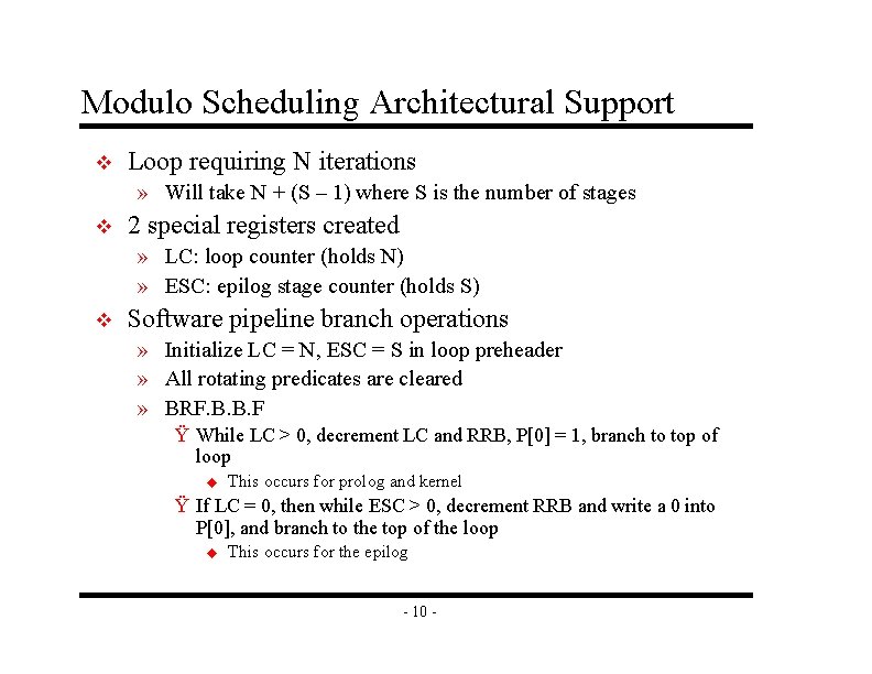
Kernel-only Code Using Rotating Predicates A 0 A 1 B 0 A 2 B 1 C 0 A B C D Bn Cn-1 Cn Dn-2 Dn-1 Dn P[0] 1 1 … 0 0 0 A if P[0] B if P[1] C if P[2] D if P[3] P referred to as the staging predicate P[1] 0 1 1 1 P[2] 0 0 1 1 P[3] 0 0 0 1 1 1 A A … -9 - B B B C C D B - C C - D D D

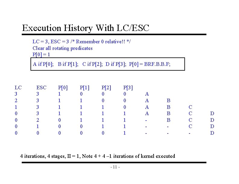
Modulo Scheduling Architectural Support v Loop requiring N iterations » Will take N + (S – 1) where S is the number of stages v 2 special registers created » LC: loop counter (holds N) » ESC: epilog stage counter (holds S) v Software pipeline branch operations » Initialize LC = N, ESC = S in loop preheader » All rotating predicates are cleared » BRF. B. B. F Ÿ While LC > 0, decrement LC and RRB, P[0] = 1, branch to top of loop u This occurs for prolog and kernel Ÿ If LC = 0, then while ESC > 0, decrement RRB and write a 0 into P[0], and branch to the top of the loop u This occurs for the epilog - 10 -

Execution History With LC/ESC LC = 3, ESC = 3 /* Remember 0 relative!! */ Clear all rotating predicates P[0] = 1 A if P[0]; B if P[1]; C if P[2]; D if P[3]; P[0] = BRF. B. B. F; LC 3 2 1 0 0 ESC 3 3 2 1 0 P[0] 1 1 0 0 0 P[1] 0 1 1 0 0 P[2] 0 0 1 1 0 P[3] 0 0 0 1 1 A A - B B - 4 iterations, 4 stages, II = 1, Note 4 + 4 – 1 iterations of kernel executed - 11 - C C - D D

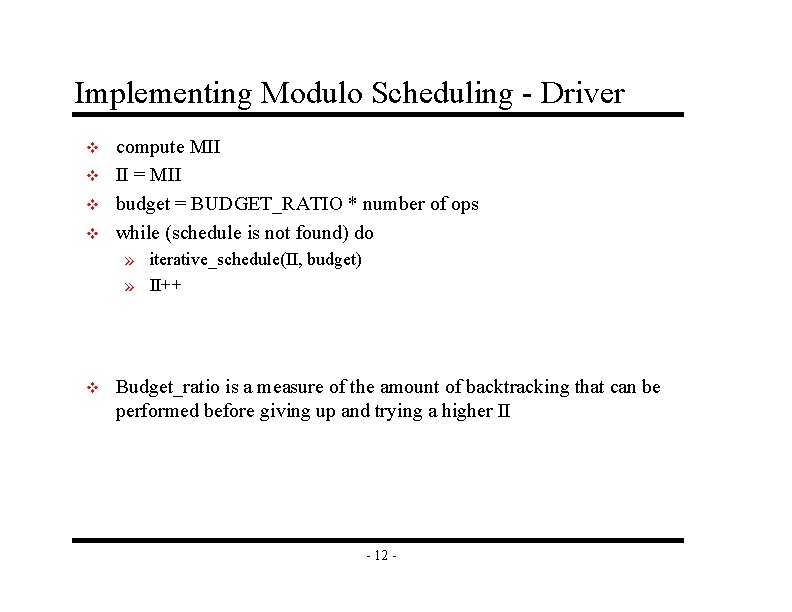
Implementing Modulo Scheduling - Driver v v compute MII II = MII budget = BUDGET_RATIO * number of ops while (schedule is not found) do » iterative_schedule(II, budget) » II++ v Budget_ratio is a measure of the amount of backtracking that can be performed before giving up and trying a higher II - 12 -

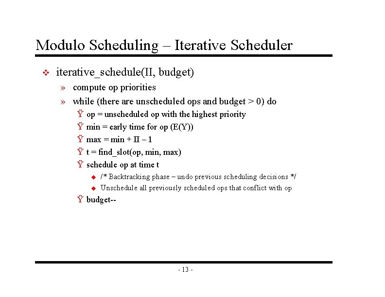
Modulo Scheduling – Iterative Scheduler v iterative_schedule(II, budget) » compute op priorities » while (there are unscheduled ops and budget > 0) do Ÿ Ÿ Ÿ op = unscheduled op with the highest priority min = early time for op (E(Y)) max = min + II – 1 t = find_slot(op, min, max) schedule op at time t u u /* Backtracking phase – undo previous scheduling decisions */ Unschedule all previously scheduled ops that conflict with op Ÿ budget-- - 13 -

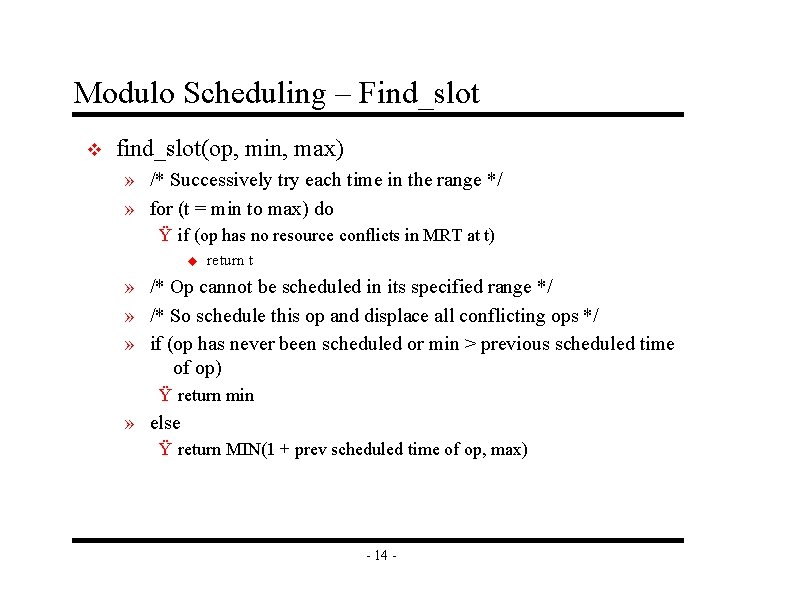
Modulo Scheduling – Find_slot v find_slot(op, min, max) » /* Successively try each time in the range */ » for (t = min to max) do Ÿ if (op has no resource conflicts in MRT at t) u return t » /* Op cannot be scheduled in its specified range */ » /* So schedule this op and displace all conflicting ops */ » if (op has never been scheduled or min > previous scheduled time of op) Ÿ return min » else Ÿ return MIN(1 + prev scheduled time of op, max) - 14 -

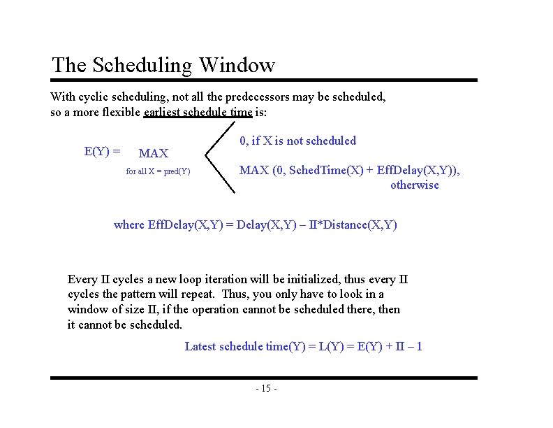
The Scheduling Window With cyclic scheduling, not all the predecessors may be scheduled, so a more flexible earliest schedule time is: E(Y) = 0, if X is not scheduled MAX for all X = pred(Y) MAX (0, Sched. Time(X) + Eff. Delay(X, Y)), otherwise where Eff. Delay(X, Y) = Delay(X, Y) – II*Distance(X, Y) Every II cycles a new loop iteration will be initialized, thus every II cycles the pattern will repeat. Thus, you only have to look in a window of size II, if the operation cannot be scheduled there, then it cannot be scheduled. Latest schedule time(Y) = L(Y) = E(Y) + II – 1 - 15 -

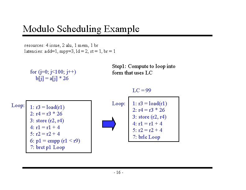
Modulo Scheduling Example resources: 4 issue, 2 alu, 1 mem, 1 br latencies: add=1, mpy=3, ld = 2, st = 1, br = 1 for (j=0; j<100; j++) b[j] = a[j] * 26 Step 1: Compute to loop into form that uses LC LC = 99 Loop: 1: r 3 = load(r 1) 2: r 4 = r 3 * 26 3: store (r 2, r 4) 4: r 1 = r 1 + 4 5: r 2 = r 2 + 4 6: p 1 = cmpp (r 1 < r 9) 7: brct p 1 Loop: - 16 - 1: r 3 = load(r 1) 2: r 4 = r 3 * 26 3: store (r 2, r 4) 4: r 1 = r 1 + 4 5: r 2 = r 2 + 4 7: brlc Loop

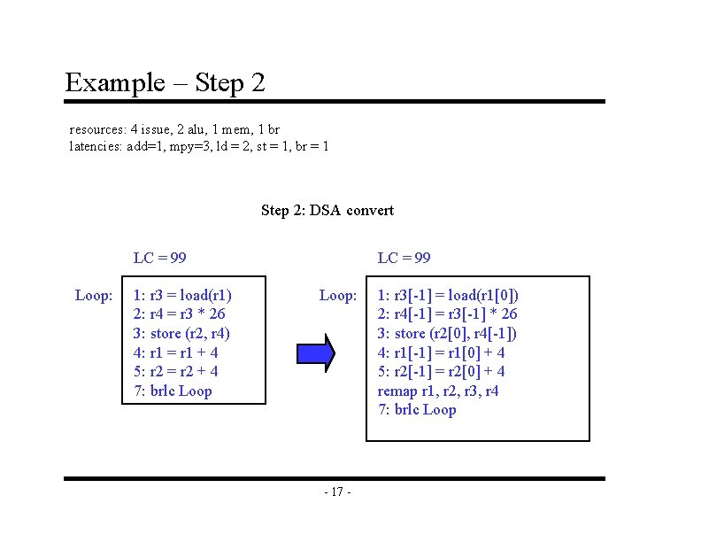
Example – Step 2 resources: 4 issue, 2 alu, 1 mem, 1 br latencies: add=1, mpy=3, ld = 2, st = 1, br = 1 Step 2: DSA convert LC = 99 Loop: 1: r 3 = load(r 1) 2: r 4 = r 3 * 26 3: store (r 2, r 4) 4: r 1 = r 1 + 4 5: r 2 = r 2 + 4 7: brlc Loop LC = 99 Loop: - 17 - 1: r 3[-1] = load(r 1[0]) 2: r 4[-1] = r 3[-1] * 26 3: store (r 2[0], r 4[-1]) 4: r 1[-1] = r 1[0] + 4 5: r 2[-1] = r 2[0] + 4 remap r 1, r 2, r 3, r 4 7: brlc Loop

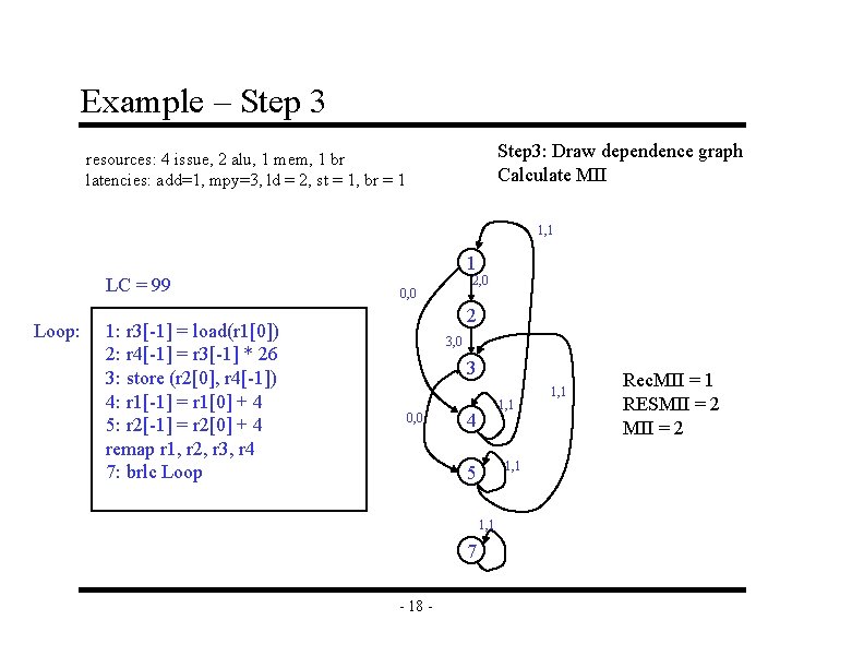
Example – Step 3: Draw dependence graph Calculate MII resources: 4 issue, 2 alu, 1 mem, 1 br latencies: add=1, mpy=3, ld = 2, st = 1, br = 1 1, 1 1 LC = 99 Loop: 1: r 3[-1] = load(r 1[0]) 2: r 4[-1] = r 3[-1] * 26 3: store (r 2[0], r 4[-1]) 4: r 1[-1] = r 1[0] + 4 5: r 2[-1] = r 2[0] + 4 remap r 1, r 2, r 3, r 4 7: brlc Loop 2, 0 0, 0 2 3, 0 3 0, 0 1, 1 4 1, 1 5 1, 1 7 - 18 - 1, 1 Rec. MII = 1 RESMII = 2

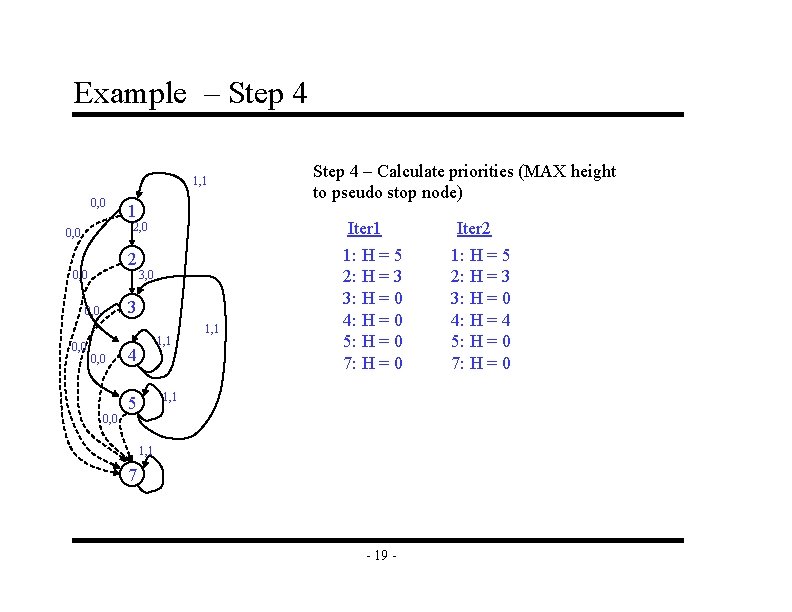
Example – Step 4 1, 1 0, 0 1 2, 0 0, 0 2 0, 0 3 0, 0 1, 1 4 1, 1 Step 4 – Calculate priorities (MAX height to pseudo stop node) Iter 1 1: H = 5 2: H = 3 3: H = 0 4: H = 0 5: H = 0 7: H = 0 1, 1 5 0, 0 1, 1 7 - 19 - Iter 2 1: H = 5 2: H = 3 3: H = 0 4: H = 4 5: H = 0 7: H = 0

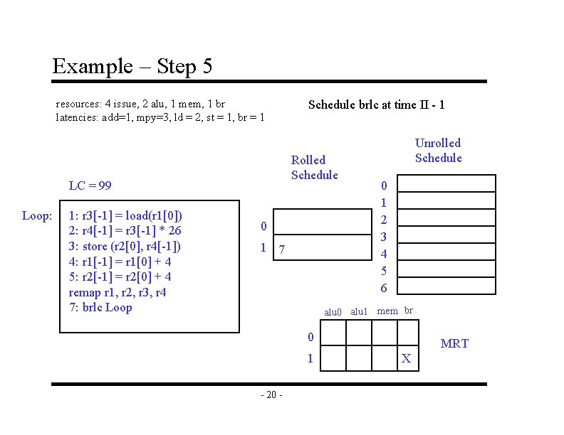
Example – Step 5 resources: 4 issue, 2 alu, 1 mem, 1 br latencies: add=1, mpy=3, ld = 2, st = 1, br = 1 Rolled Schedule LC = 99 Loop: 1: r 3[-1] = load(r 1[0]) 2: r 4[-1] = r 3[-1] * 26 3: store (r 2[0], r 4[-1]) 4: r 1[-1] = r 1[0] + 4 5: r 2[-1] = r 2[0] + 4 remap r 1, r 2, r 3, r 4 7: brlc Loop Schedule brlc at time II - 1 0 1 7 Unrolled Schedule 0 1 2 3 4 5 6 alu 0 alu 1 mem br 0 1 - 20 - MRT X

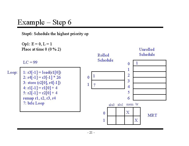
Example – Step 6: Schedule the highest priority op Op 1: E = 0, L = 1 Place at time 0 (0 % 2) Rolled Schedule LC = 99 Loop: 1: r 3[-1] = load(r 1[0]) 2: r 4[-1] = r 3[-1] * 26 3: store (r 2[0], r 4[-1]) 4: r 1[-1] = r 1[0] + 4 5: r 2[-1] = r 2[0] + 4 remap r 1, r 2, r 3, r 4 7: brlc Loop 0 1 1 7 Unrolled Schedule 0 1 2 3 4 5 6 1 alu 0 alu 1 mem br 0 1 - 21 - X MRT X

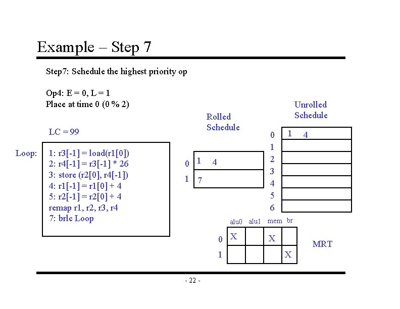
Example – Step 7: Schedule the highest priority op Op 4: E = 0, L = 1 Place at time 0 (0 % 2) Rolled Schedule LC = 99 Loop: 1: r 3[-1] = load(r 1[0]) 2: r 4[-1] = r 3[-1] * 26 3: store (r 2[0], r 4[-1]) 4: r 1[-1] = r 1[0] + 4 5: r 2[-1] = r 2[0] + 4 remap r 1, r 2, r 3, r 4 7: brlc Loop 0 1 4 1 7 Unrolled Schedule 0 1 2 3 4 5 6 1 4 alu 0 alu 1 mem br 0 X 1 - 22 - X MRT X

Example – Step 8: Schedule the highest priority op Op 2: E = 2, L = 3 Place at time 2 (2 % 2) Rolled Schedule LC = 99 Loop: 1: r 3[-1] = load(r 1[0]) 2: r 4[-1] = r 3[-1] * 26 3: store (r 2[0], r 4[-1]) 4: r 1[-1] = r 1[0] + 4 5: r 2[-1] = r 2[0] + 4 remap r 1, r 2, r 3, r 4 7: brlc Loop Unrolled Schedule 0 1 4 0 1 2 3 4 5 6 2 1 7 1 4 2 alu 0 alu 1 mem br 0 X 1 - 23 - X X MRT X

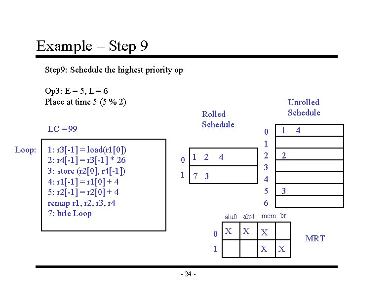
Example – Step 9: Schedule the highest priority op Op 3: E = 5, L = 6 Place at time 5 (5 % 2) Rolled Schedule LC = 99 Loop: 1: r 3[-1] = load(r 1[0]) 2: r 4[-1] = r 3[-1] * 26 3: store (r 2[0], r 4[-1]) 4: r 1[-1] = r 1[0] + 4 5: r 2[-1] = r 2[0] + 4 remap r 1, r 2, r 3, r 4 7: brlc Loop Unrolled Schedule 0 1 2 3 4 5 6 4 1 7 3 1 4 2 3 alu 0 alu 1 mem br 0 X 1 - 24 - X X X MRT X

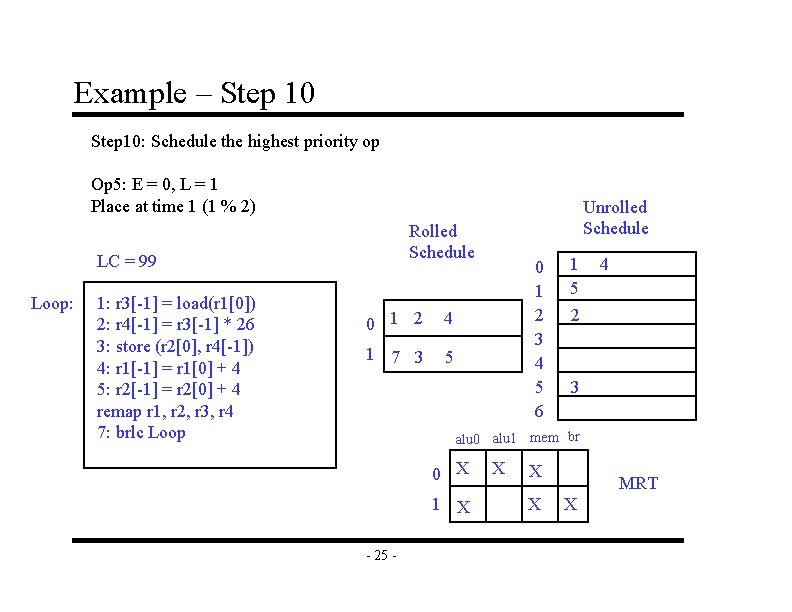
Example – Step 10: Schedule the highest priority op Op 5: E = 0, L = 1 Place at time 1 (1 % 2) Rolled Schedule LC = 99 Loop: 1: r 3[-1] = load(r 1[0]) 2: r 4[-1] = r 3[-1] * 26 3: store (r 2[0], r 4[-1]) 4: r 1[-1] = r 1[0] + 4 5: r 2[-1] = r 2[0] + 4 remap r 1, r 2, r 3, r 4 7: brlc Loop Unrolled Schedule 0 1 2 4 1 7 3 5 0 1 2 3 4 5 6 1 5 2 4 3 alu 0 alu 1 mem br 0 X 1 X - 25 - X X X MRT X

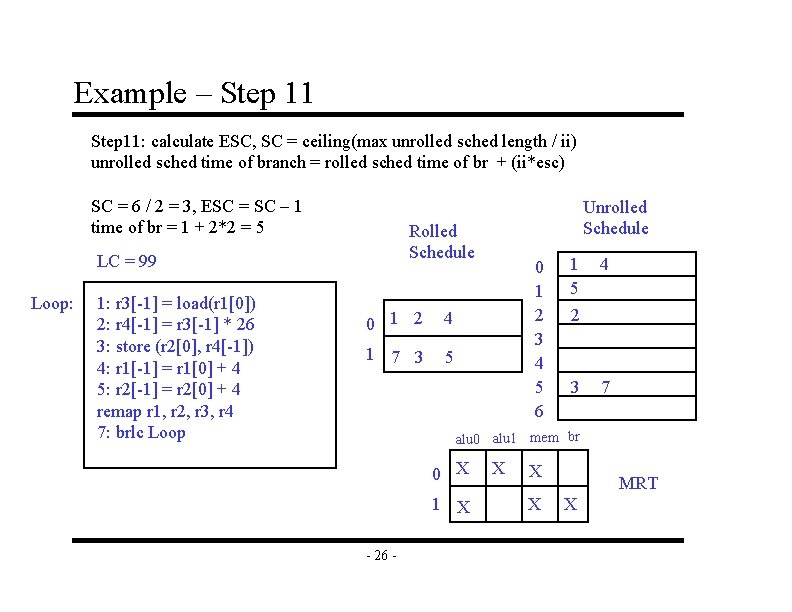
Example – Step 11: calculate ESC, SC = ceiling(max unrolled sched length / ii) unrolled sched time of branch = rolled sched time of br + (ii*esc) SC = 6 / 2 = 3, ESC = SC – 1 time of br = 1 + 2*2 = 5 Rolled Schedule LC = 99 Loop: 1: r 3[-1] = load(r 1[0]) 2: r 4[-1] = r 3[-1] * 26 3: store (r 2[0], r 4[-1]) 4: r 1[-1] = r 1[0] + 4 5: r 2[-1] = r 2[0] + 4 remap r 1, r 2, r 3, r 4 7: brlc Loop Unrolled Schedule 0 1 2 4 1 7 3 5 0 1 2 3 4 5 6 1 5 2 4 3 7 alu 0 alu 1 mem br 0 X 1 X - 26 - X X X MRT X

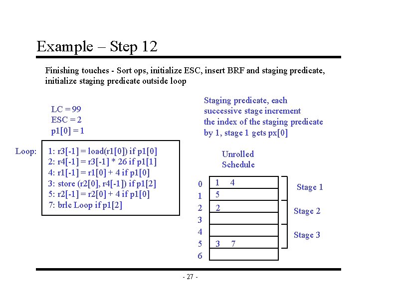
Example – Step 12 Finishing touches - Sort ops, initialize ESC, insert BRF and staging predicate, initialize staging predicate outside loop Staging predicate, each successive stage increment the index of the staging predicate by 1, stage 1 gets px[0] LC = 99 ESC = 2 p 1[0] = 1 Loop: 1: r 3[-1] = load(r 1[0]) if p 1[0] 2: r 4[-1] = r 3[-1] * 26 if p 1[1] 4: r 1[-1] = r 1[0] + 4 if p 1[0] 3: store (r 2[0], r 4[-1]) if p 1[2] 5: r 2[-1] = r 2[0] + 4 if p 1[0] 7: brlc Loop if p 1[2] Unrolled Schedule 0 1 2 3 4 5 6 - 27 - 1 5 2 3 4 Stage 1 Stage 2 7 Stage 3

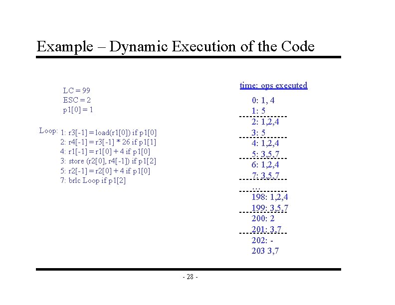
Example – Dynamic Execution of the Code time: ops executed LC = 99 ESC = 2 p 1[0] = 1 0: 1, 4 1: 5 2: 1, 2, 4 3: 5 4: 1, 2, 4 5: 3, 5, 7 6: 1, 2, 4 7: 3, 5, 7 … 198: 1, 2, 4 199: 3, 5, 7 200: 2 201: 3, 7 202: 203 3, 7 Loop: 1: r 3[-1] = load(r 1[0]) if p 1[0] 2: r 4[-1] = r 3[-1] * 26 if p 1[1] 4: r 1[-1] = r 1[0] + 4 if p 1[0] 3: store (r 2[0], r 4[-1]) if p 1[2] 5: r 2[-1] = r 2[0] + 4 if p 1[0] 7: brlc Loop if p 1[2] - 28 -

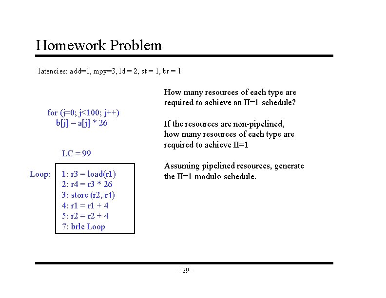
Homework Problem latencies: add=1, mpy=3, ld = 2, st = 1, br = 1 How many resources of each type are required to achieve an II=1 schedule? for (j=0; j<100; j++) b[j] = a[j] * 26 LC = 99 Loop: 1: r 3 = load(r 1) 2: r 4 = r 3 * 26 3: store (r 2, r 4) 4: r 1 = r 1 + 4 5: r 2 = r 2 + 4 7: brlc Loop If the resources are non-pipelined, how many resources of each type are required to achieve II=1 Assuming pipelined resources, generate the II=1 modulo schedule. - 29 -

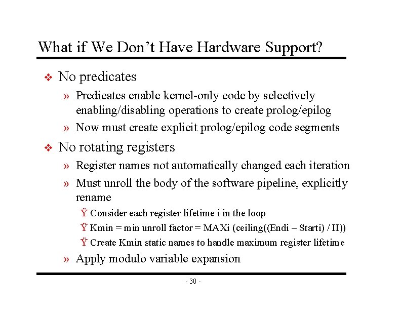
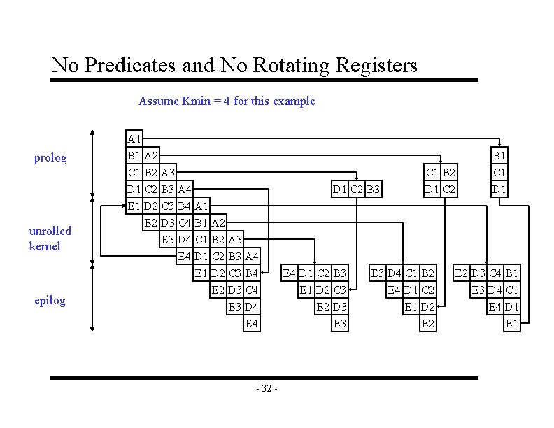
What if We Don’t Have Hardware Support? v No predicates » Predicates enable kernel-only code by selectively enabling/disabling operations to create prolog/epilog » Now must create explicit prolog/epilog code segments v No rotating registers » Register names not automatically changed each iteration » Must unroll the body of the software pipeline, explicitly rename Ÿ Consider each register lifetime i in the loop Ÿ Kmin = min unroll factor = MAXi (ceiling((Endi – Starti) / II)) Ÿ Create Kmin static names to handle maximum register lifetime » Apply modulo variable expansion - 30 -

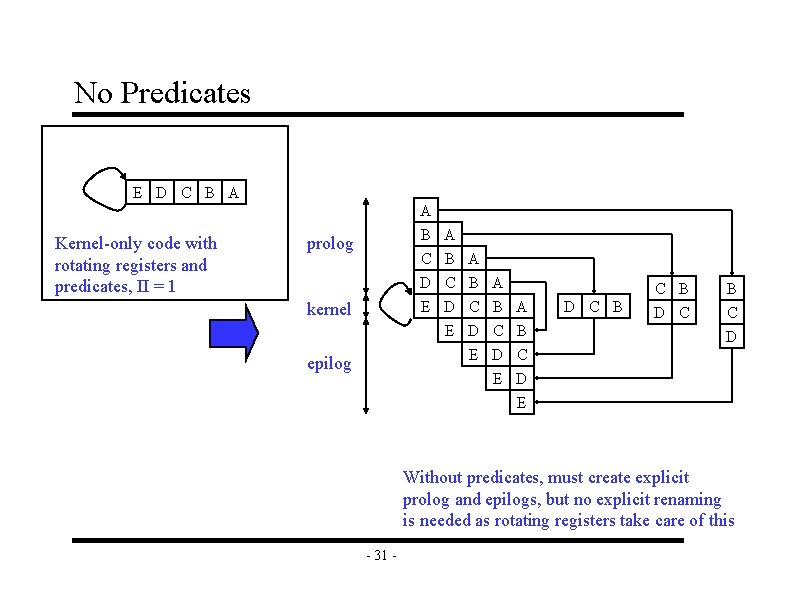
No Predicates E D C B A Kernel-only code with rotating registers and predicates, II = 1 A B A C B A prolog D C B E D C E D E kernel epilog A B C D E D C B C D Without predicates, must create explicit prolog and epilogs, but no explicit renaming is needed as rotating registers take care of this - 31 -

No Predicates and No Rotating Registers Assume Kmin = 4 for this example prolog unrolled kernel epilog A 1 B 1 A 2 C 1 B 2 A 3 D 1 C 2 B 3 A 4 E 1 D 2 C 3 B 4 A 1 E 2 D 3 C 4 B 1 A 2 E 3 D 4 C 1 B 2 A 3 E 4 D 1 C 2 B 3 A 4 E 1 D 2 C 3 B 4 E 2 D 3 C 4 E 3 D 4 E 4 - 32 - D 1 C 2 B 3 E 4 D 1 C 2 B 3 E 1 D 2 C 3 E 2 D 3 E 3 C 1 B 2 B 1 C 1 D 1 C 2 D 1 E 3 D 4 C 1 B 2 E 4 D 1 C 2 E 1 D 2 E 2 D 3 C 4 B 1 E 3 D 4 C 1 E 4 D 1 E 1