EE 359 Wireless Communications Announcements and Course Summary

EE 359: Wireless Communications Announcements and Course Summary

Announcements l l Last HW and bonus HW questions due Sunday 12/10 at 4 pm (no late HWs). Final projects must be posted 12/9 (Sat) at midnight. 25 bonus points for course evaluations (online) Final 12/13/2017, 12: 15 -3: 15 pm in Thornton 102 (here) Covers Chapters 9, 10, 12, 13. 1 -13. 2, 13. 4, 14. 1 -14. 4, 15. 1 -15. 4 (+ earlier chps) l Similar format to MT, but longer: open book, notes. l If you need a book or calculator, let us know by 12/8 (Fri) l Practice finals posted (10 bonus points). Turn in for l

OHs leading up to final exam l Mine l This week: today after class, Fri 12 -1 pm & by appt. l Next week: Sun 12/10: 5 -6 pm, Tue 12/11 10: 30 -12 & by appt. l TAs: l l l l Thursday, 12/7, 5 -6 pm Milind OH Thursday, 12/7, 6 -7 pm Milind Email OH Saturday, 12/9, 2 -4 pm Tom OH (HW 8 + Exam questions) Monday, 12/11, 2 -4 pm Final review Monday, 12/11, 4 -6 pm Tom OH Tuesday, 12/12 2 -4 pm Milind OH Wednesday, 12/13, 9: 30 am-11: 30 am, Tom OH

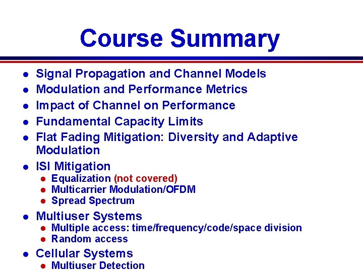
Course Summary l l l Signal Propagation and Channel Models Modulation and Performance Metrics Impact of Channel on Performance Fundamental Capacity Limits Flat Fading Mitigation: Diversity and Adaptive Modulation ISI Mitigation l l Multiuser Systems l l l Equalization (not covered) Multicarrier Modulation/OFDM Spread Spectrum Multiple access: time/frequency/code/space division Random access Cellular Systems l Multiuser Detection

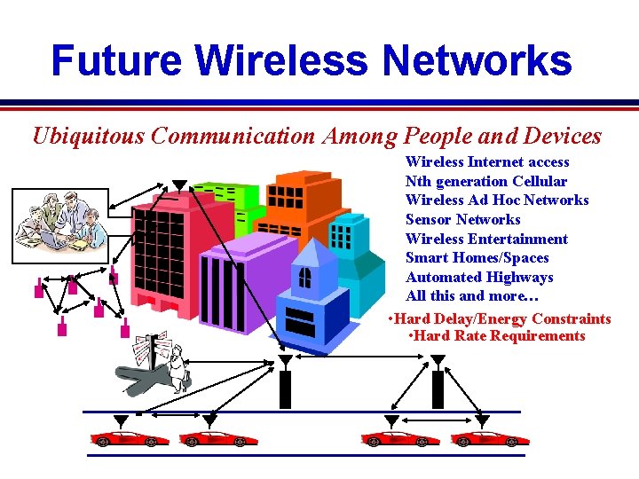
Future Wireless Networks Ubiquitous Communication Among People and Devices Wireless Internet access Nth generation Cellular Wireless Ad Hoc Networks Sensor Networks Wireless Entertainment Smart Homes/Spaces Automated Highways All this and more… • Hard Delay/Energy Constraints • Hard Rate Requirements

Design Challenges l Wireless channels are a difficult and capacity -limited broadcast communications medium l Traffic patterns, user locations, and network conditions are constantly changing l Applications are heterogeneous with hard constraints that must be met by the network l Energy, delay, and rate constraints change design principles across all layers of the protocol stack

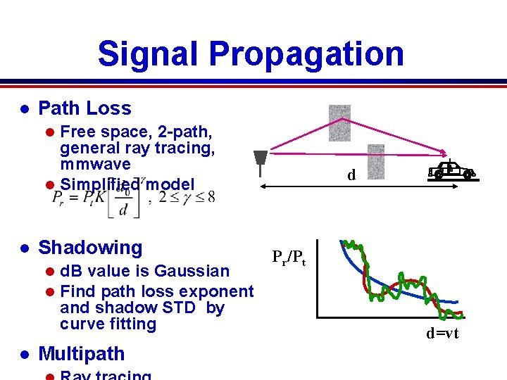
Signal Propagation l Path Loss Free space, 2 -path, general ray tracing, mmwave l Simplified model l l Shadowing l l l d. B value is Gaussian Find path loss exponent and shadow STD by curve fitting Multipath d Pr/Pt d=vt

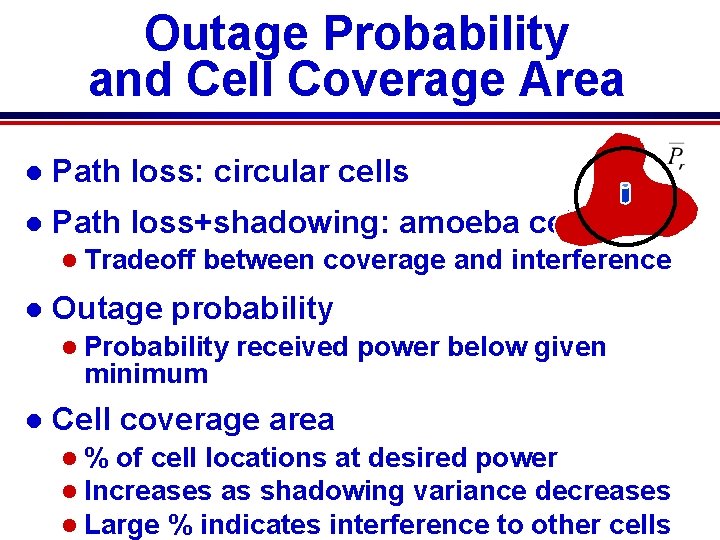
Outage Probability and Cell Coverage Area l Path loss: circular cells l Path loss+shadowing: amoeba cells l Tradeoff l between coverage and interference Outage probability l Probability minimum l received power below given Cell coverage area l % of cell locations at desired power l Increases as shadowing variance decreases l Large % indicates interference to other cells

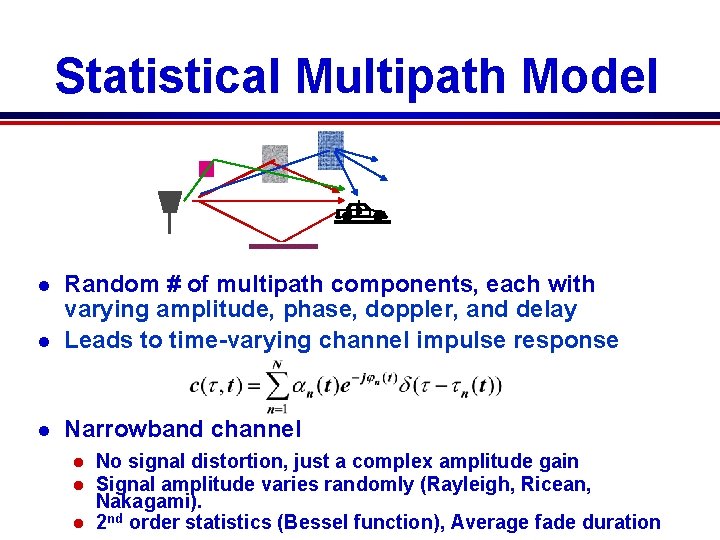
Statistical Multipath Model l Random # of multipath components, each with varying amplitude, phase, doppler, and delay Leads to time-varying channel impulse response l Narrowband channel l No signal distortion, just a complex amplitude gain Signal amplitude varies randomly (Rayleigh, Ricean, Nakagami). l 2 nd order statistics (Bessel function), Average fade duration l l

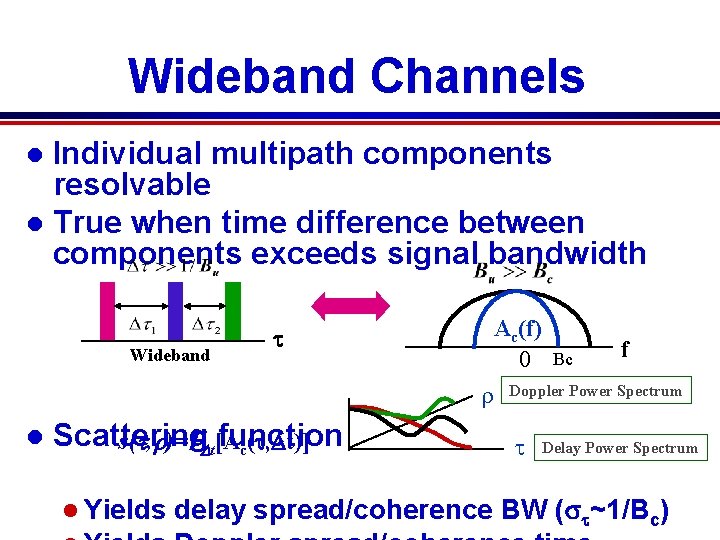
Wideband Channels Individual multipath components resolvable l True when time difference between components exceeds signal bandwidth l Wideband Ac(f) 0 t r l Scattering function s(t, r)=FDt[A c(t, Dt)] l Yields Bc f Doppler Power Spectrum t Delay Power Spectrum delay spread/coherence BW (st~1/Bc)

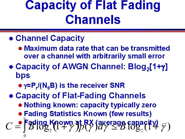
Capacity of Flat Fading Channels l Channel Capacity l Maximum data rate that can be transmitted over a channel with arbitrarily small error l Capacity of AWGN Channel: Blog 2[1+g] bps l g=Pr/(N 0 B) l is the receiver SNR Capacity of Flat-Fading Channels l Nothing known: capacity typically zero l Fading Statistics Known (few results) l Fading Known at RX (average capacity)

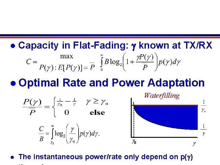
l Capacity in Flat-Fading: g known at TX/RX l Optimal Rate and Power Adaptation Waterfilling 1 g g 0 l g The instantaneous power/rate only depend on p(g)

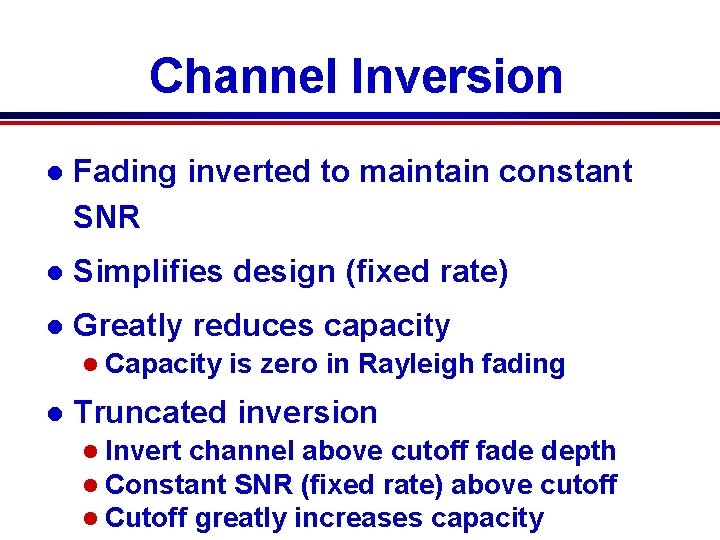
Channel Inversion l Fading inverted to maintain constant SNR l Simplifies design (fixed rate) l Greatly reduces capacity l Capacity l is zero in Rayleigh fading Truncated inversion l Invert channel above cutoff fade depth l Constant SNR (fixed rate) above cutoff l Cutoff greatly increases capacity

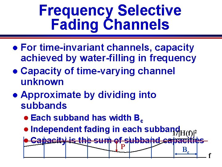
Frequency Selective Fading Channels For time-invariant channels, capacity achieved by water-filling in frequency l Capacity of time-varying channel unknown l Approximate by dividing into subbands l l Each subband has width Bc l Independent fading in each subband 1/|H(f)|2 l Capacity is the sum of subband capacities P Bc f

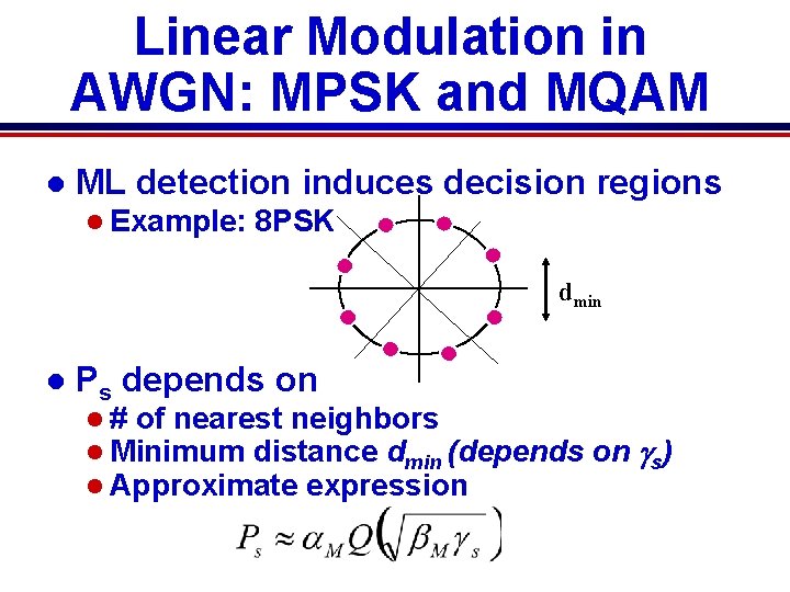
Linear Modulation in AWGN: MPSK and MQAM l ML detection induces decision regions l Example: 8 PSK dmin l Ps depends on l # of nearest neighbors l Minimum distance dmin (depends l Approximate expression on gs)

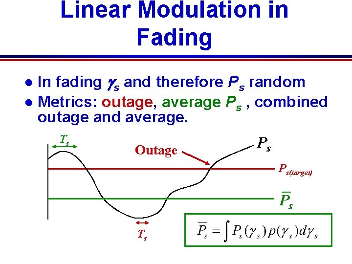
Linear Modulation in Fading In fading gs and therefore Ps random l Metrics: outage, average Ps , combined outage and average. l Ts Outage Ps Ps(target) Ps Ts

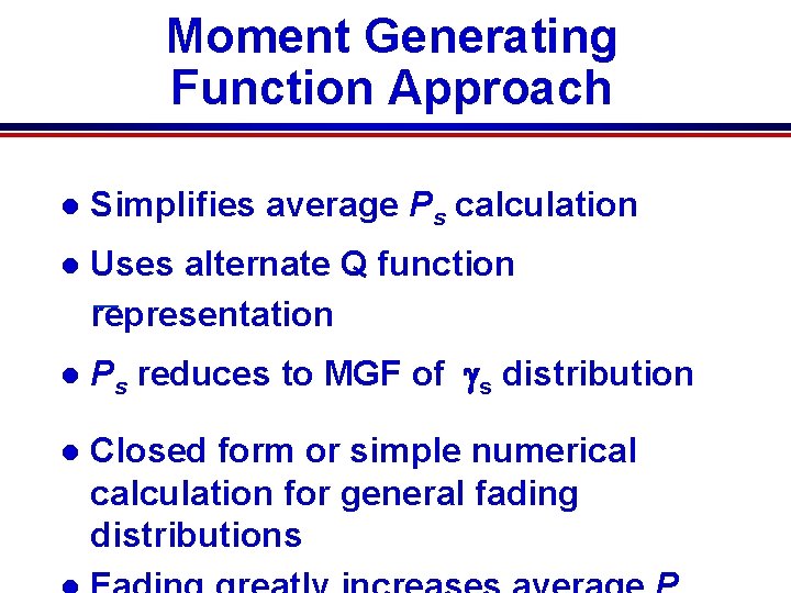
Moment Generating Function Approach l Simplifies average Ps calculation l Uses alternate Q function representation l Ps reduces to MGF of gs distribution l Closed form or simple numerical calculation for general fading distributions

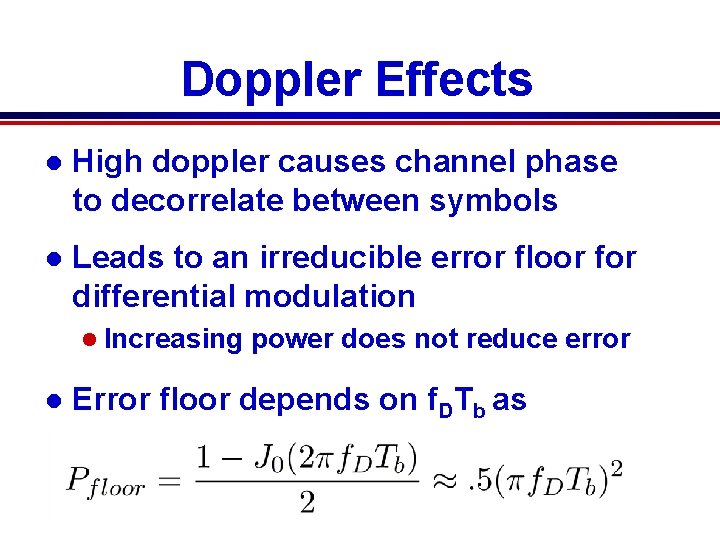
Doppler Effects l High doppler causes channel phase to decorrelate between symbols l Leads to an irreducible error floor for differential modulation l Increasing l power does not reduce error Error floor depends on f. DTb as

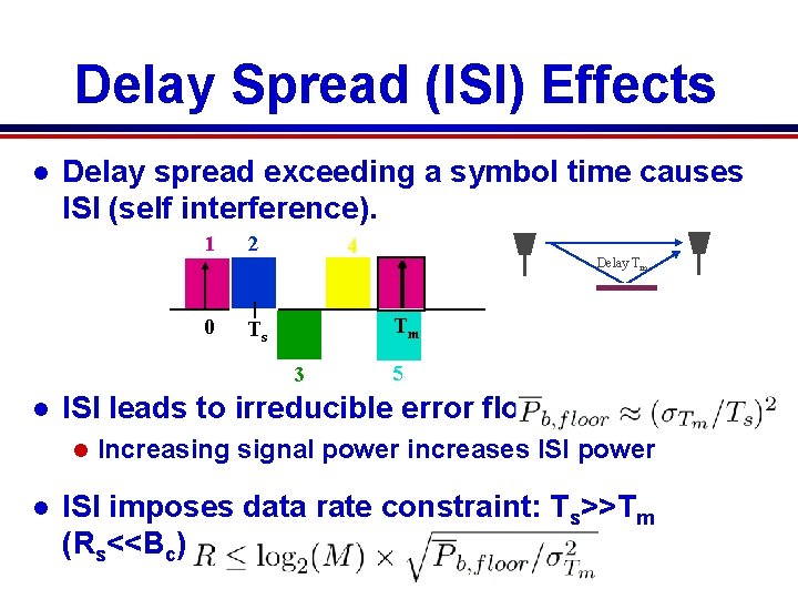
Delay Spread (ISI) Effects l Delay spread exceeding a symbol time causes ISI (self interference). 1 2 0 Ts 4 Tm 3 l 5 ISI leads to irreducible error floor: l l Delay Tm Increasing signal power increases ISI power ISI imposes data rate constraint: Ts>>Tm (Rs<<Bc)

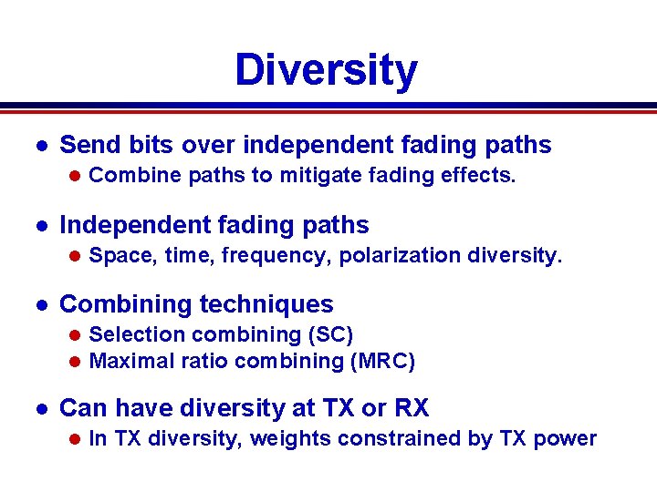
Diversity l Send bits over independent fading paths l l Independent fading paths l l Space, time, frequency, polarization diversity. Combining techniques l l l Combine paths to mitigate fading effects. Selection combining (SC) Maximal ratio combining (MRC) Can have diversity at TX or RX l In TX diversity, weights constrained by TX power

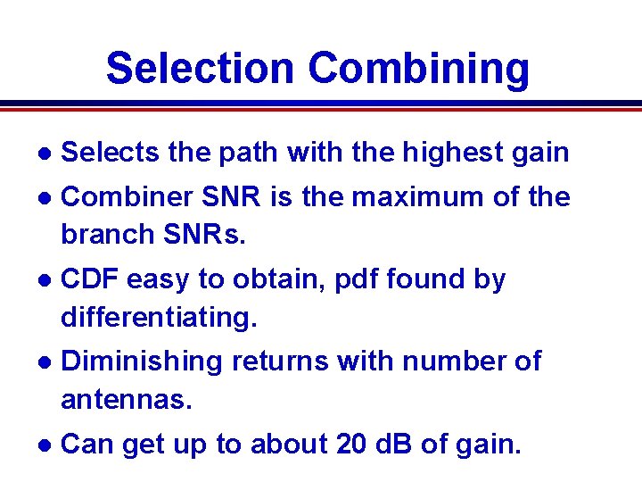
Selection Combining l Selects the path with the highest gain l Combiner SNR is the maximum of the branch SNRs. l CDF easy to obtain, pdf found by differentiating. l Diminishing returns with number of antennas. l Can get up to about 20 d. B of gain.

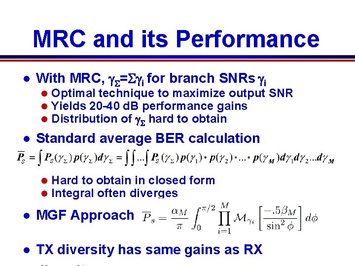
MRC and its Performance l With MRC, g = gi for branch SNRs gi l l Optimal technique to maximize output SNR Yields 20 -40 d. B performance gains Distribution of g hard to obtain Standard average BER calculation s s l l s Hard to obtain in closed form Integral often diverges l MGF Approach: l TX diversity has same gains as RX

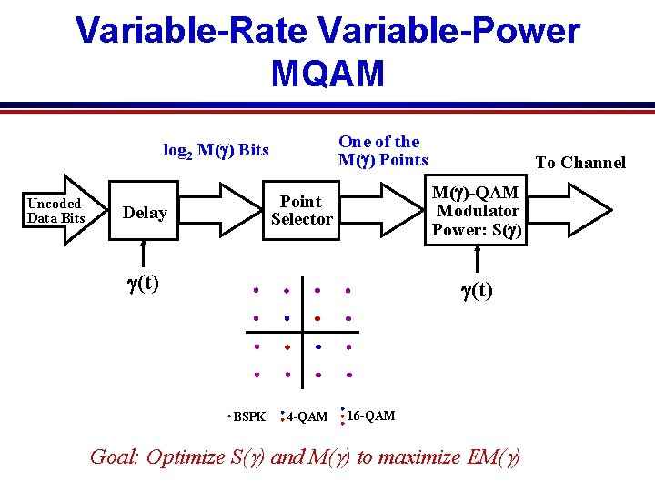
Variable-Rate Variable-Power MQAM One of the M(g) Points log 2 M(g) Bits Uncoded Data Bits M(g)-QAM Modulator Power: S(g) Point Selector Delay To Channel g(t) BSPK 4 -QAM 16 -QAM Goal: Optimize S(g) and M(g) to maximize EM(g)

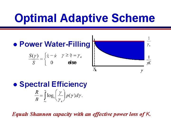
Optimal Adaptive Scheme l Power Water-Filling gk l g Spectral Efficiency g Equals Shannon capacity with an effective power loss of K.

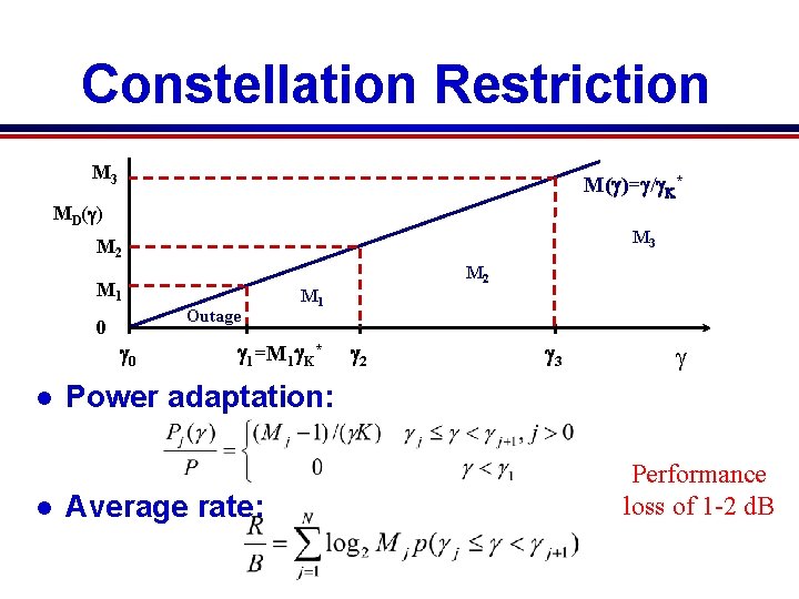
Constellation Restriction M 3 M(g)=g/g. K* MD(g) M 3 M 2 M 1 Outage 0 g 0 l l M 1 g 1=M 1 g. K* g 2 g 3 g Power adaptation: Average rate: Performance loss of 1 -2 d. B

Practical Constraints (not on final) l Constant power restriction l Another l Constellation updates l Need l 1 -2 d. B loss constellation constant over 10 -100 Ts Estimation error and delay l Lead to imperfect CSIT (assume perfect CSIR) l Causes mismatch between channel and rate

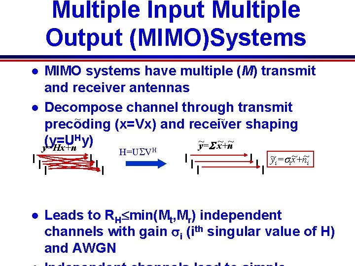
Multiple Input Multiple Output (MIMO)Systems MIMO systems have multiple (M) transmit and receiver antennas l Decompose channel through transmit ~ ~ precoding (x=Vx) and receiver shaping Hy) ~ ~ ~ (y=U y=S x+n y=Hx+n l H=USVH l ~ ~ ~ yi=six+n i Leads to RH min(Mt, Mr) independent channels with gain si (ith singular value of H) and AWGN

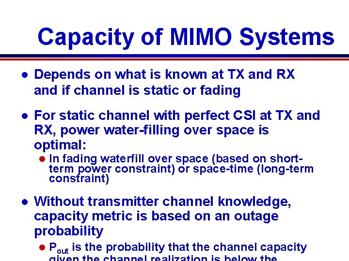
Capacity of MIMO Systems l Depends on what is known at TX and RX and if channel is static or fading l For static channel with perfect CSI at TX and RX, power water-filling over space is optimal: l l In fading waterfill over space (based on shortterm power constraint) or space-time (long-term constraint) Without transmitter channel knowledge, capacity metric is based on an outage probability l Pout is the probability that the channel capacity

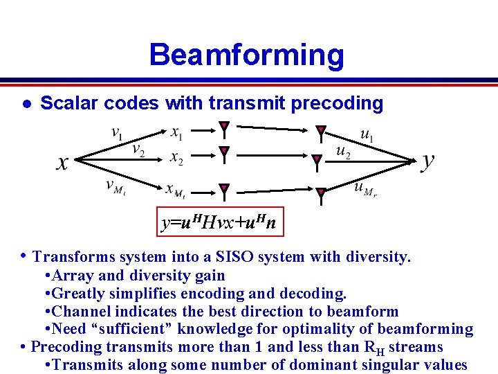
Beamforming l Scalar codes with transmit precoding y=u. HHvx+u. Hn • Transforms system into a SISO system with diversity. • Array and diversity gain • Greatly simplifies encoding and decoding. • Channel indicates the best direction to beamform • Need “sufficient” knowledge for optimality of beamforming • Precoding transmits more than 1 and less than RH streams • Transmits along some number of dominant singular values

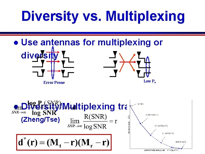
Diversity vs. Multiplexing l Use antennas for multiplexing or diversity Error Prone l Low Pe Diversity/Multiplexing tradeoffs (Zheng/Tse)

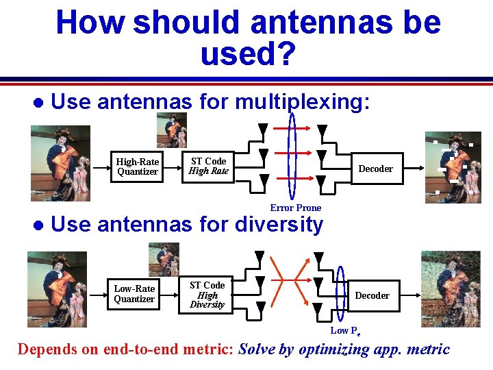
How should antennas be used? l Use antennas for multiplexing: High-Rate Quantizer ST Code High Rate Decoder Error Prone l Use antennas for diversity Low-Rate Quantizer ST Code High Diversity Decoder Low Pe Depends on end-to-end metric: Solve by optimizing app. metric

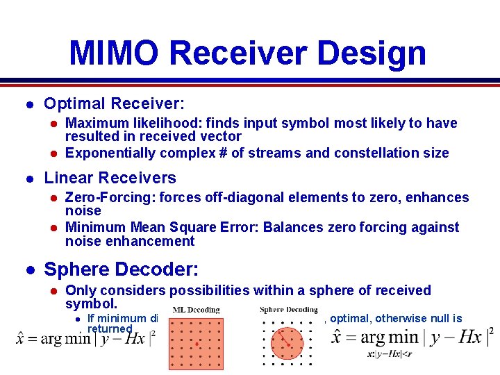
MIMO Receiver Design l Optimal Receiver: Maximum likelihood: finds input symbol most likely to have resulted in received vector l Exponentially complex # of streams and constellation size l l Linear Receivers Zero-Forcing: forces off-diagonal elements to zero, enhances noise l Minimum Mean Square Error: Balances zero forcing against noise enhancement l l Sphere Decoder: l Only considers possibilities within a sphere of received symbol. l If minimum distance symbol is within sphere, optimal, otherwise null is returned

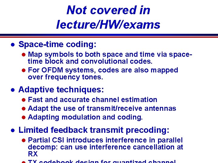
Not covered in lecture/HW/exams l Space-time coding: Map symbols to both space and time via spacetime block and convolutional codes. l For OFDM systems, codes are also mapped over frequency tones. l l Adaptive techniques: l l Fast and accurate channel estimation Adapt the use of transmit/receive antennas Adapting modulation and coding. Limited feedback transmit precoding: l Partial CSI introduces interference in parallel decomp: can use interference cancellation at RX

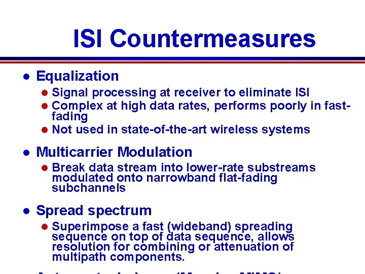
ISI Countermeasures l Equalization Signal processing at receiver to eliminate ISI Complex at high data rates, performs poorly in fastfading l Not used in state-of-the-art wireless systems l l l Multicarrier Modulation l l Break data stream into lower-rate substreams modulated onto narrowband flat-fading subchannels Spread spectrum l Superimpose a fast (wideband) spreading sequence on top of data sequence, allows resolution for combining or attenuation of multipath components.

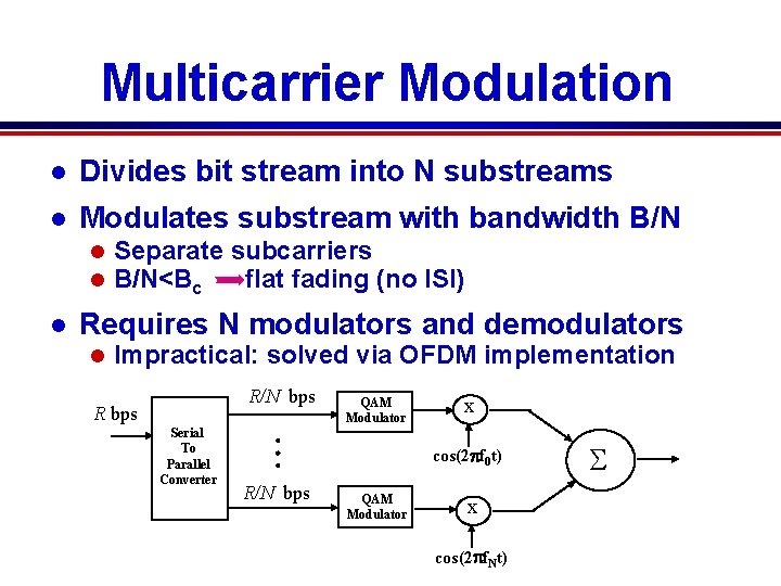
Multicarrier Modulation l Divides bit stream into N substreams l Modulates substream with bandwidth B/N l l l Separate subcarriers B/N<Bc flat fading (no ISI) Requires N modulators and demodulators l Impractical: solved via OFDM implementation R/N bps R bps Serial To Parallel Converter QAM Modulator x cos(2 pf 0 t) R/N bps QAM Modulator x cos(2 pf. Nt) S

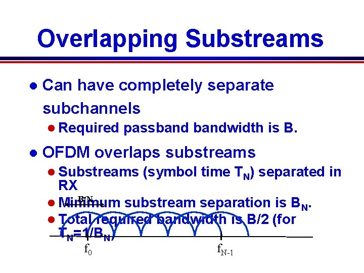
Overlapping Substreams l Can have completely separate subchannels l Required l passbandwidth is B. OFDM overlaps substreams l Substreams (symbol time TN) separated in RX B/N l Minimum substream separation is BN. l Total required bandwidth is B/2 (for TN=1/BN) f 0 f. N-1

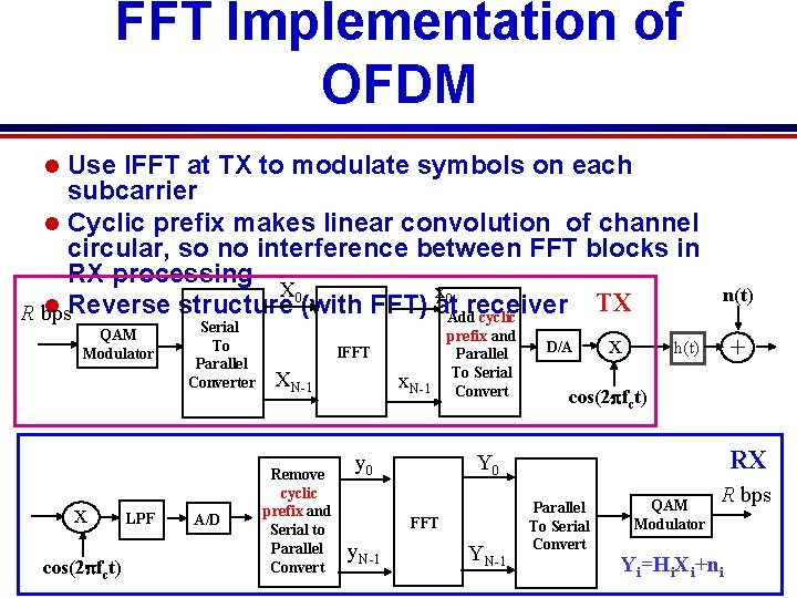
FFT Implementation of OFDM Use IFFT at TX to modulate symbols on each subcarrier l Cyclic prefix makes linear convolution of channel circular, so no interference between FFT blocks in RX processing X 0 x 0 TX l Reverse structure (with FFT) at. Addreceiver R bps cyclic l QAM Modulator x cos(2 pfct) LPF Serial To Parallel Converter A/D IFFT XN-1 Remove cyclic prefix and Serial to Parallel Convert x. N-1 prefix and Parallel To Serial Convert x + h(t) cos(2 pfct) RX Y 0 y 0 FFT y. N-1 D/A n(t) YN-1 Parallel To Serial Convert QAM Modulator R bps Yi=Hi. Xi+ni

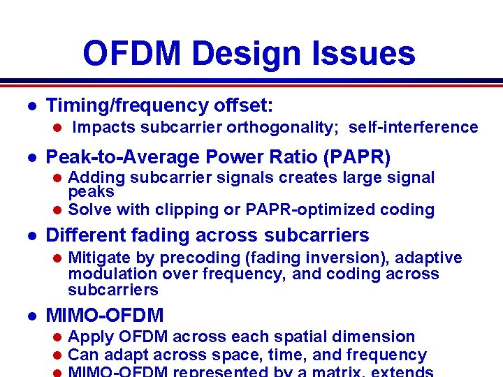
OFDM Design Issues l Timing/frequency offset: l l Impacts subcarrier orthogonality; self-interference Peak-to-Average Power Ratio (PAPR) Adding subcarrier signals creates large signal peaks l Solve with clipping or PAPR-optimized coding l l Different fading across subcarriers l l Mitigate by precoding (fading inversion), adaptive modulation over frequency, and coding across subcarriers MIMO-OFDM l l Apply OFDM across each spatial dimension Can adapt across space, time, and frequency

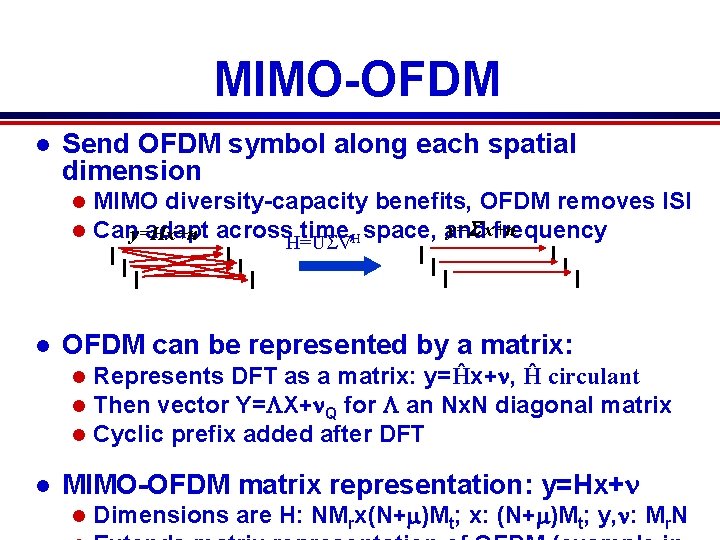
MIMO-OFDM l Send OFDM symbol along each spatial dimension l l l OFDM can be represented by a matrix: l l MIMO diversity-capacity benefits, OFDM removes ISI y=S x+n Cany=Hx+n adapt across. H=USV time, Hspace, and frequency Represents DFT as a matrix: y=Ĥx+n, Ĥ circulant Then vector Y=LX+n. Q for L an Nx. N diagonal matrix Cyclic prefix added after DFT MIMO-OFDM matrix representation: y=Hx+n l Dimensions are H: NMrx(N+m)Mt; x: (N+m)Mt; y, n: Mr. N

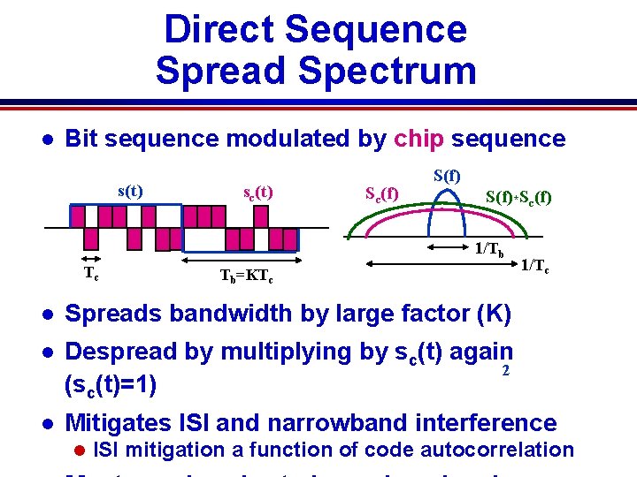
Direct Sequence Spread Spectrum l Bit sequence modulated by chip sequence s(t) sc(t) Sc(f) S(f)*Sc(f) 1/Tb Tc Tb=KTc 1/Tc l Spreads bandwidth by large factor (K) l Despread by multiplying by sc(t) again 2 (sc(t)=1) l Mitigates ISI and narrowband interference l ISI mitigation a function of code autocorrelation

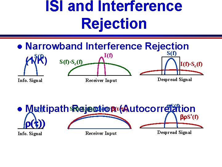
ISI and Interference Rejection l Narrowband Interference Rejection S(f) I(f) S(f) (1/K) S(f)*Sc(f) Info. Signal l Receiver Input Despread Signal a. S(f) *Sc(f)[ad(t)+b(t-t)] S(f) Multipath Rejection (Autocorrelation br. S’(f) r(t)) Info. Signal Receiver Input Despread Signal

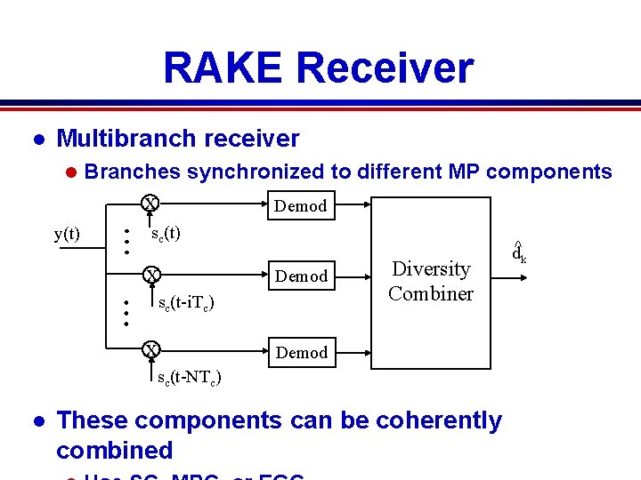
RAKE Receiver l Multibranch receiver l y(t) Branches synchronized to different MP components x Demod sc(t) x Demod sc(t-i. Tc) x Diversity Combiner Demod sc(t-NTc) l These components can be coherently combined d^k

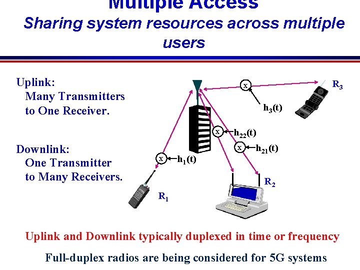
Multiple Access Sharing system resources across multiple users Uplink: Many Transmitters to One Receiver. h 3(t) x Downlink: One Transmitter to Many Receivers. R 3 x h 22(t) x x h 1(t) h 21(t) R 2 R 1 Uplink and Downlink typically duplexed in time or frequency Full-duplex radios are being considered for 5 G systems

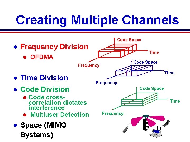
Creating Multiple Channels Code Space l Frequency Division l Time OFDMA Code Space Frequency l Time Division l Code Division Code crosscorrelation dictates interference l Multiuser Detection Time Frequency Code Space l l 7 C 29822. 033 -Cimini-9/97 Space (MIMO Systems) Time Frequency

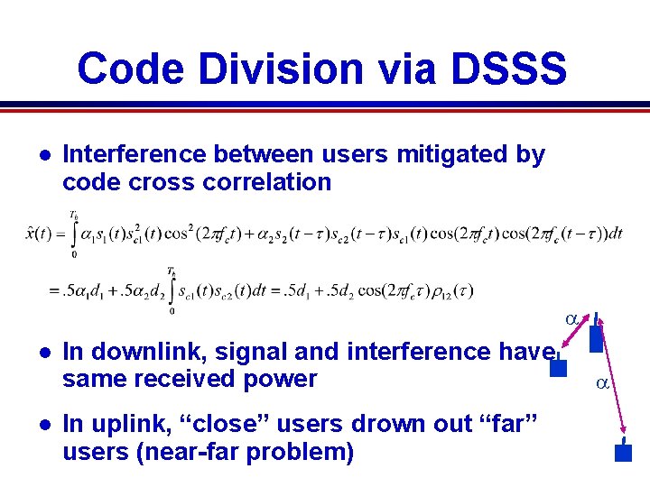
Code Division via DSSS l Interference between users mitigated by code cross correlation a l l In downlink, signal and interference have same received power In uplink, “close” users drown out “far” users (near-far problem) a

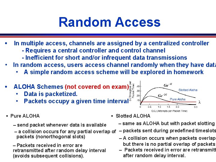
Random Access • In multiple access, channels are assigned by a centralized controller - Requires a central controller and control channel - Inefficient for short and/or infrequent data transmissions • In random access, users access channel randomly when they have data • A simple random access scheme will be explored in homework • ALOHA Schemes (not covered on exam) • Data is packetized. • Packets occupy a given time interval • Pure ALOHA • Slotted ALOHA – same as ALOHA but with packet slotting – send packet whenever data is available – a collision occurs for any partial overlap of – packets sent during predefined timeslots packets (nonorthogonal slots) – A collision occurs when packets overlap, but there is no partial overlap of packets – Packets received in error are retransmitted after random delay interval. (avoids subsequent collisions).

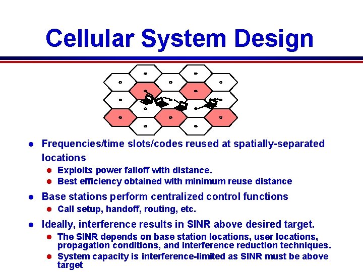
Cellular System Design l Frequencies/time slots/codes reused at spatially-separated locations l l l Base stations perform centralized control functions l l Call setup, handoff, routing, etc. Ideally, interference results in SINR above desired target. The SINR depends on base station locations, user locations, propagation conditions, and interference reduction techniques. l System capacity is interference-limited as SINR must be above target l 8 C 32810. 43 -Cimini-7/98 Exploits power falloff with distance. Best efficiency obtained with minimum reuse distance

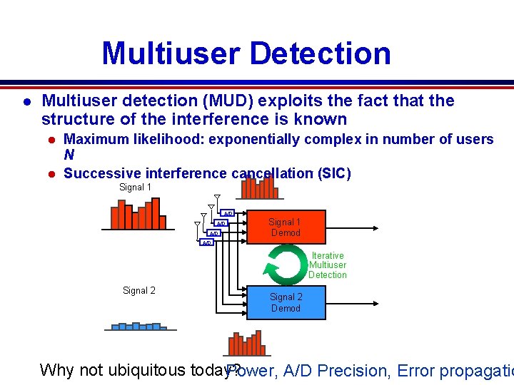
Multiuser Detection l Multiuser detection (MUD) exploits the fact that the structure of the interference is known Maximum likelihood: exponentially complex in number of users N l Successive interference cancellation (SIC) l - Signal 1 = A/D A/D Signal 1 Demod A/D Iterative Multiuser Detection Signal 2 Demod - = Why not ubiquitous today? Power, A/D Precision, Error propagatio

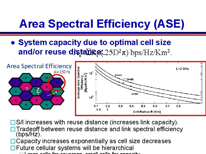
Area Spectral Efficiency (ASE) l System capacity due to optimal cell size and/or reuse distance: Ae=SRi/(. 25 D 2 p) bps/Hz/Km 2. Area Spectral Efficiency A=. 25 D 2 p �S/I increases with reuse distance (increases link capacity). �Tradeoff between reuse distance and link spectral efficiency (bps/Hz). �Capacity increases exponentially as cell size decreases �Future cellular systems will be hierarchical

Megathemes of EE 359 l The wireless vision poses great technical challenges l The wireless channel greatly impedes performance l l l Compensate for flat fading with diversity or adaptive mod. l l Low fundamental capacity; Channel is randomly time-varying. Flat fading and ISI must be compensated for. MIMO provides diversity and/or multiplexing gain A plethora of ISI compensation techniques exist Various tradeoffs in performance, complexity, and implementation. l OFDM is the dominant technique; works well with MIMO, basis for 4 G/5 G Cellular/Wi. Fi due to adaptivity over time/space/frequency l l Sharing spectrum among multiple users a major challenge