Discrimination and Classification The Optimal Classification Rule Suppose

Discrimination and Classification

The Optimal Classification Rule Suppose that the data x 1, … , xp has joint density function f(x 1, … , xp ; q) where q is either q 1 or q 2. Let g(x 1, … , xp) = f(x 1, … , xn ; q 1) and h(x 1, … , xp) = f(x 1, … , xn ; q 2) We want to make the decision D 1: q = q 1 (g is the correct distribution) against D 2: q = q 2 (h is the correct distribution)

then the optimal regions (minimizing ECM, expected cost of misclassification) for making the decisions D 1 and D 2 respectively are C 1 and C 2 and where

Fishers Linear Discriminant Function. Suppose that x 1, … , xp is either data from a p-variate Normal distribution with mean vector: The covariance matrix S is the same for both populations p 1 and p 2.

We make the decision D 1 : population is p 1 if where and

In the case where the populations are unknown but estimated from data Fisher’s linear discriminant function

The function Is called Fisher’s linear discriminant function

Discrimination of p-variate Normal distributions (unequal Covariance matrices) Suppose that x 1, … , xp is either data from a p-variate Normal distribution with mean vector: and covariance matrices, S 1 and S 2 respectively.

The optimal rule states that we should classify into populations p 1 and p 2 using: That is make the decision D 1 : population is p 1 if l ≥ k

or where and

Summarizing we make the decision to classify in population p 1 if: where and

Discrimination of p-variate Normal distributions (unequal Covariance matrices)

Classification or Cluster Analysis Have data from one or several populations

Situation • Have multivariate (or univariate) data from one or several populations (the number of populations is unknown) • Want to determine the number of populations and identify the populations

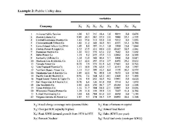
Example

Hierarchical Clustering Methods The following are the steps in the agglomerative Hierarchical clustering algorithm for grouping N objects (items or variables). 1. 2. 3. Start with N clusters, each consisting of a single entity and an N X N symmetric matrix (table) of distances (or similarities) D = (dij). Search the distance matrix for the nearest (most similar) pair of clusters. Let the distance between the "most similar" clusters U and V be d. UV. Merge clusters U and V. Label the newly formed cluster (UV). Update the entries in the distance matrix by a) b) deleting the rows and columns corresponding to clusters U and V and adding a row and column giving the distances between cluster (UV) and the remaining clusters.

4. Repeat steps 2 and 3 a total of N-1 times. (All objects will be a single cluster a termination of this algorithm. ) Record the identity of clusters that are merged and the levels (distances or similarities) at which the mergers take place.

Different methods of computing inter-cluster distance

Example To illustrate the single linkage algorithm, we consider the hypothetical distance matrix between pairs of five objects given below:

Treating each object as a cluster, the clustering begins by merging the two closest items (3 & 5). To implement the next level of clustering we need to compute the distances between cluster (35) and the remaining objects: d(35)1 = min{3, 11} = 3 d(35)2 = min{7, 10} = 7 d(35)4 = min{9, 8} = 8 The new distance matrix becomes:

The new distance matrix becomes: The next two closest clusters ((35) & 1) are merged to form cluster (135). Distances between this cluster and the remaining clusters become:

Distances between this cluster and the remaining clusters become: d(135)2 = min{7, 9} = 7 d(135)4 = min{8, 6} = 6 The distance matrix now becomes: Continuing the next two closest clusters (2 & 4) are merged to form cluster (24).

Distances between this cluster and the remaining clusters become: d(135)(24) = min{d(135)2, d(135)4)= min{7, 6} = 6 The final distance matrix now becomes: At the final step clusters (135) and (24) are merged to form the single cluster (12345) of all five items.

The results of this algorithm can be summarized graphically on the following "dendogram"

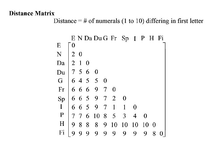
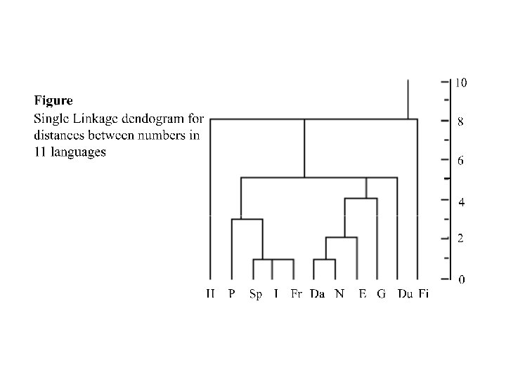
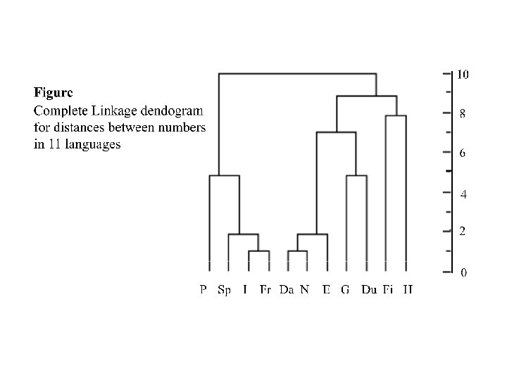
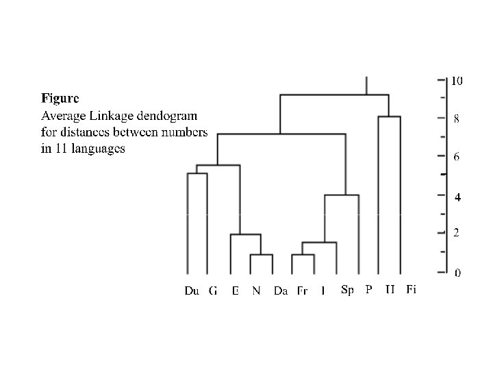
Dendograms for clustering the 11 languages on the basis of the ten numerals

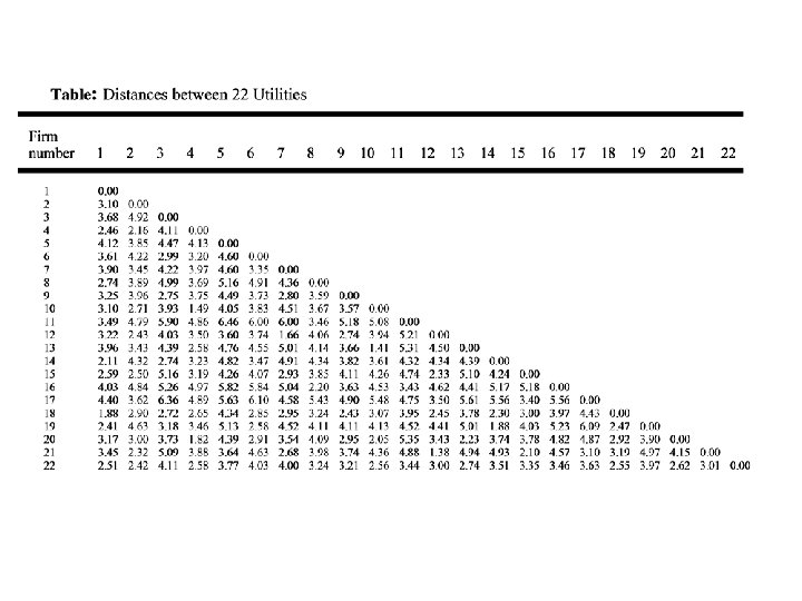
Dendogram Cluster Analysis of N=22 Utility companies Euclidean distance, Average Linkage

Dendogram Cluster Analysis of N=22 Utility companies Euclidean distance, Single Linkage