Digital Communications Fredrik Rusek Chapter 10 adaptive equalization

Digital Communications Fredrik Rusek Chapter 10, adaptive equalization and more Proakis-Salehi

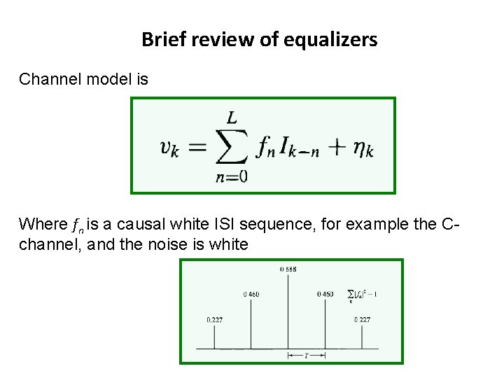
Brief review of equalizers Channel model is Where fn is a causal white ISI sequence, for example the Cchannel, and the noise is white

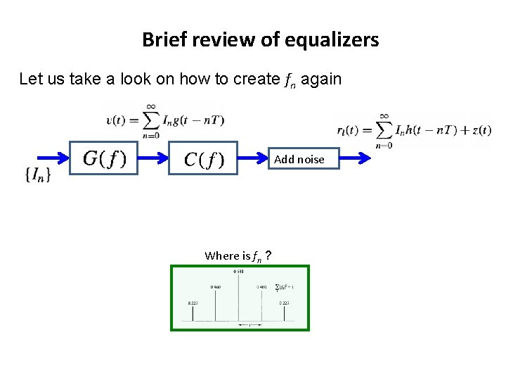
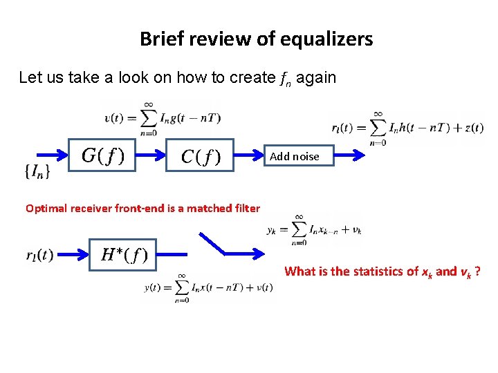
Brief review of equalizers Let us take a look on how to create fn again Add noise Where is fn ?

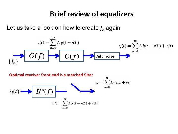
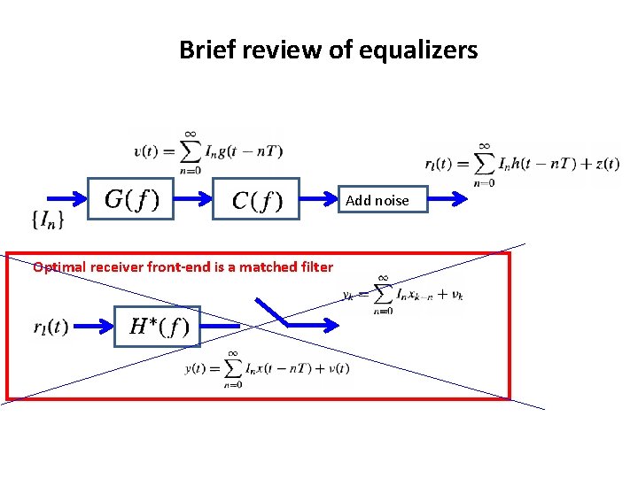
Brief review of equalizers Let us take a look on how to create fn again Add noise Optimal receiver front-end is a matched filter

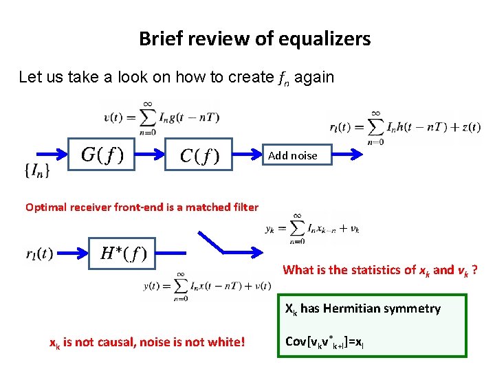
Brief review of equalizers Let us take a look on how to create fn again Add noise Optimal receiver front-end is a matched filter What is the statistics of xk and vk ?

Brief review of equalizers Let us take a look on how to create fn again Add noise Optimal receiver front-end is a matched filter What is the statistics of xk and vk ? Xk has Hermitian symmetry xk is not causal, noise is not white! Cov[vkv*k+l]=xl

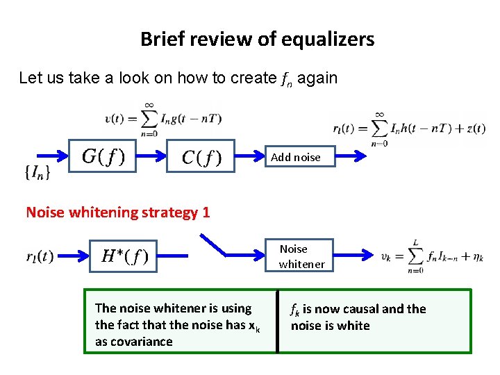
Brief review of equalizers Let us take a look on how to create fn again Add noise Noise whitening strategy 1 Noise whitener The noise whitener is using the fact that the noise has xk as covariance fk is now causal and the noise is white

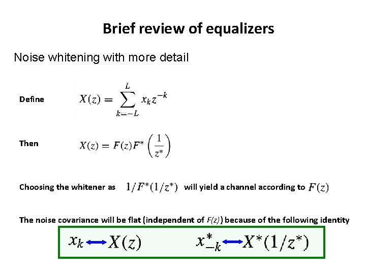
Brief review of equalizers Noise whitening with more detail Define Then Choosing the whitener as will yield a channel according to The noise covariance will be flat (independent of F(z)) because of the following identity

Brief review of equalizers Noise whitening strategy 2. Important. • • • In practice, one seldomly sees the matched filter followed by the whitener. Hardware implementation of MF is fixed, and cannot depend on the channel How to build the front-end? • Desires: – Should be optimal – Should generate white noise at output

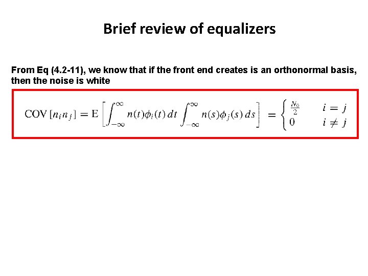
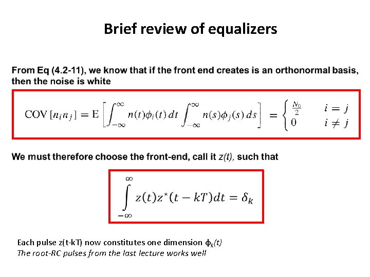
Brief review of equalizers From Eq (4. 2 -11), we know that if the front end creates is an orthonormal basis, then the noise is white

Brief review of equalizers • Each pulse z(t-k. T) now constitutes one dimension φk(t) The root-RC pulses from the last lecture works well

Brief review of equalizers Noise whitening strategy 2. Important. • • • In practice, one seldomly sees the matched filter followed by the whitener. Hardware implementation of MF is fixed, and cannot depend on the channel How to build the front-end? • Desires: – Should be optimal – Should generate white noise at output OK! But how to guarantee optimality?

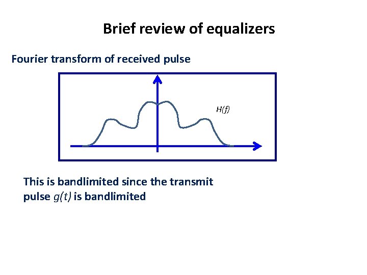
Brief review of equalizers Fourier transform of received pulse H(f) This is bandlimited since the transmit pulse g(t) is bandlimited

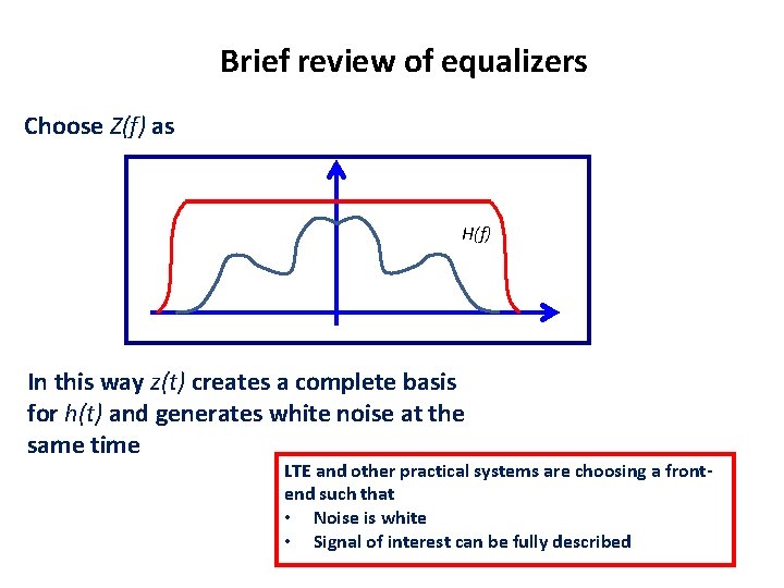
Brief review of equalizers Choose Z(f) as H(f) In this way z(t) creates a complete basis for h(t) and generates white noise at the same time LTE and other practical systems are choosing a frontend such that • Noise is white • Signal of interest can be fully described

Brief review of equalizers Add noise Optimal receiver front-end is a matched filter

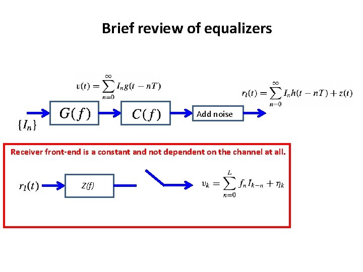
Brief review of equalizers Add noise Receiver front-end is a constant and not dependent on the channel at all. Z(f)

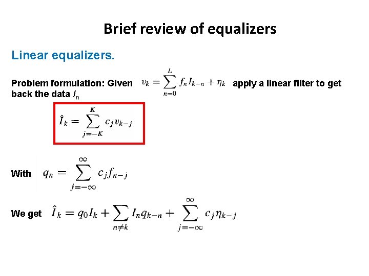
Brief review of equalizers Linear equalizers. Problem formulation: Given back the data In With We get apply a linear filter to get

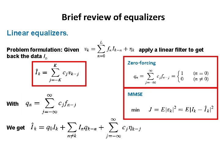
Brief review of equalizers Linear equalizers. Problem formulation: Given back the data In apply a linear filter to get Zero-forcing MMSE With We get min

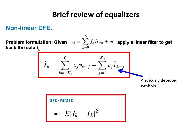
Brief review of equalizers Non-linear DFE. Problem formulation: Given back the data Ik apply a linear filter to get Previously detected symbols DFE - MMSE min

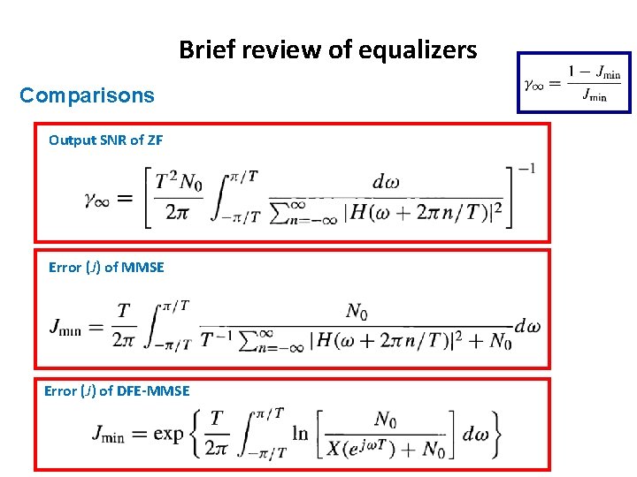
Brief review of equalizers Comparisons Output SNR of ZF Error (J) of MMSE Error (J) of DFE-MMSE

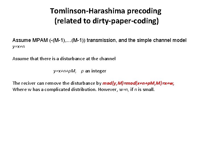
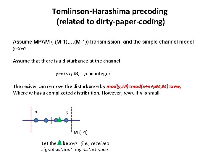
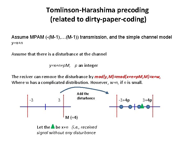
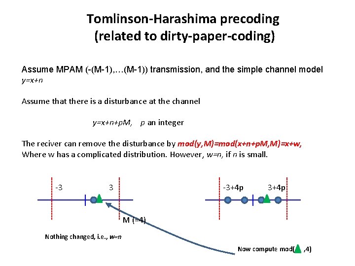
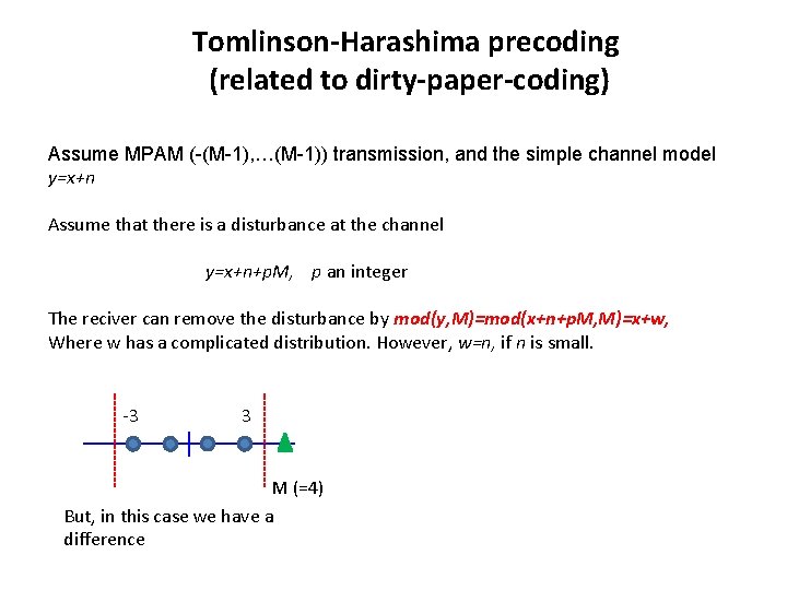
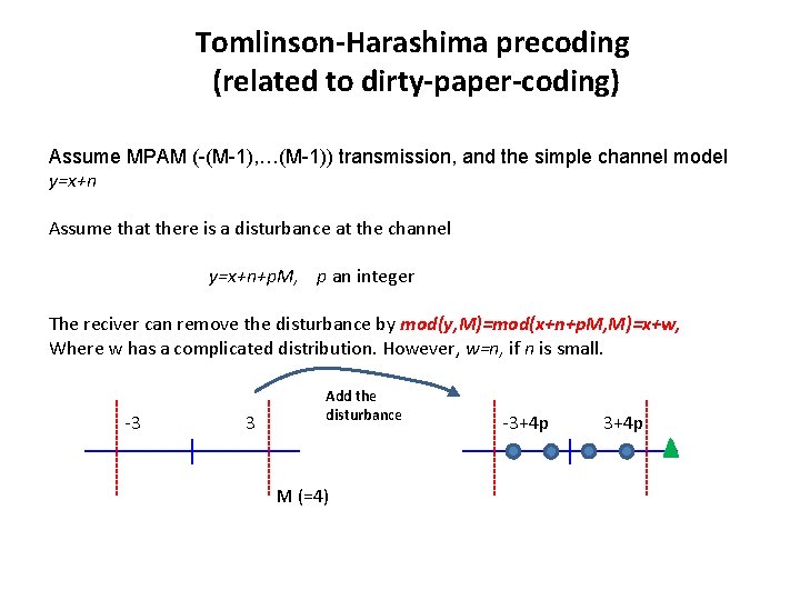
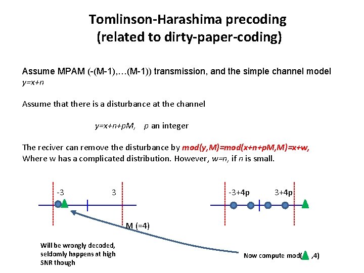
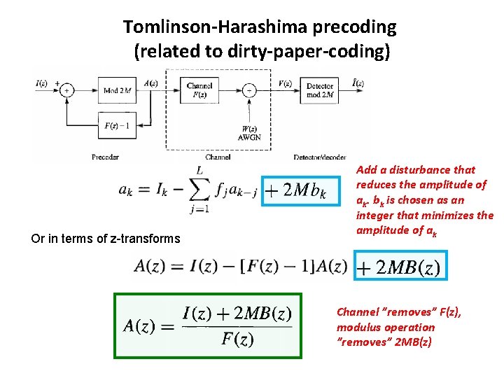
Tomlinson-Harashima precoding (related to dirty-paper-coding) Assume MPAM (-(M-1), …(M-1)) transmission, and the simple channel model y=x+n Assume that there is a disturbance at the channel y=x+n+p. M, p an integer The reciver can remove the disturbance by mod(y, M)=mod(x+n+p. M, M)=x+w, Where w has a complicated distribution. However, w=n, if n is small.

Tomlinson-Harashima precoding (related to dirty-paper-coding) Assume MPAM (-(M-1), …(M-1)) transmission, and the simple channel model y=x+n Assume that there is a disturbance at the channel y=x+n+p. M, p an integer The reciver can remove the disturbance by mod(y, M)=mod(x+n+p. M, M)=x+w, Where w has a complicated distribution. However, w=n, if n is small. -3 3 M (=4) Let the be x+n (i. e. , received signal without any disturbance

Tomlinson-Harashima precoding (related to dirty-paper-coding) Assume MPAM (-(M-1), …(M-1)) transmission, and the simple channel model y=x+n Assume that there is a disturbance at the channel y=x+n+p. M, p an integer The reciver can remove the disturbance by mod(y, M)=mod(x+n+p. M, M)=x+w, Where w has a complicated distribution. However, w=n, if n is small. -3 3 Add the disturbance M (=4) Let the be x+n (i. e. , received signal without any disturbance -3+4 p

Tomlinson-Harashima precoding (related to dirty-paper-coding) Assume MPAM (-(M-1), …(M-1)) transmission, and the simple channel model y=x+n Assume that there is a disturbance at the channel y=x+n+p. M, p an integer The reciver can remove the disturbance by mod(y, M)=mod(x+n+p. M, M)=x+w, Where w has a complicated distribution. However, w=n, if n is small. -3 3 -3+4 p M (=4) Nothing changed, i. e. , w=n Now compute mod( , 4)

Tomlinson-Harashima precoding (related to dirty-paper-coding) Assume MPAM (-(M-1), …(M-1)) transmission, and the simple channel model y=x+n Assume that there is a disturbance at the channel y=x+n+p. M, p an integer The reciver can remove the disturbance by mod(y, M)=mod(x+n+p. M, M)=x+w, Where w has a complicated distribution. However, w=n, if n is small. -3 3 M (=4) But, in this case we have a difference

Tomlinson-Harashima precoding (related to dirty-paper-coding) Assume MPAM (-(M-1), …(M-1)) transmission, and the simple channel model y=x+n Assume that there is a disturbance at the channel y=x+n+p. M, p an integer The reciver can remove the disturbance by mod(y, M)=mod(x+n+p. M, M)=x+w, Where w has a complicated distribution. However, w=n, if n is small. -3 3 Add the disturbance M (=4) -3+4 p

Tomlinson-Harashima precoding (related to dirty-paper-coding) Assume MPAM (-(M-1), …(M-1)) transmission, and the simple channel model y=x+n Assume that there is a disturbance at the channel y=x+n+p. M, p an integer The reciver can remove the disturbance by mod(y, M)=mod(x+n+p. M, M)=x+w, Where w has a complicated distribution. However, w=n, if n is small. -3 3 -3+4 p M (=4) Will be wrongly decoded, seldomly happens at high SNR though Now compute mod( , 4)

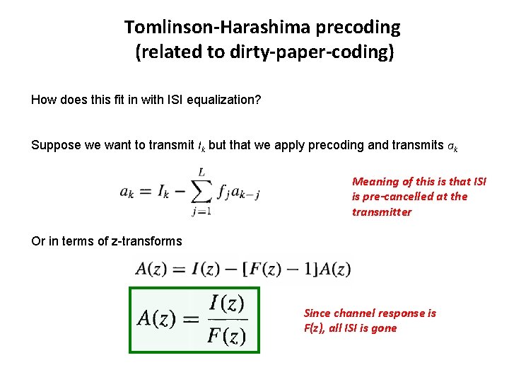
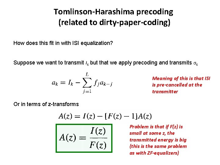
Tomlinson-Harashima precoding (related to dirty-paper-coding) How does this fit in with ISI equalization? Suppose we want to transmit Ik but that we apply precoding and transmits ak Meaning of this is that ISI is pre-cancelled at the transmitter Or in terms of z-transforms Since channel response is F(z), all ISI is gone

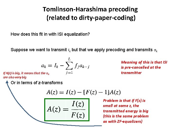
Tomlinson-Harashima precoding (related to dirty-paper-coding) How does this fit in with ISI equalization? Suppose we want to transmit Ik but that we apply precoding and transmits ak Meaning of this is that ISI is pre-cancelled at the transmitter Or in terms of z-transforms Problem is that if F(z) is small at some z, the transmitted energy is big (this is the same problem as with ZF-equalizers)

Tomlinson-Harashima precoding (related to dirty-paper-coding) How does this fit in with ISI equalization? Suppose we want to transmit Ik but that we apply precoding and transmits ak If A(z) is big, it means that the ak are also very big Meaning of this is that ISI is pre-cancelled at the transmitter Or in terms of z-transforms Problem is that if F(z) is small at some z, the transmitted energy is big (this is the same problem as with ZF-equalizers)

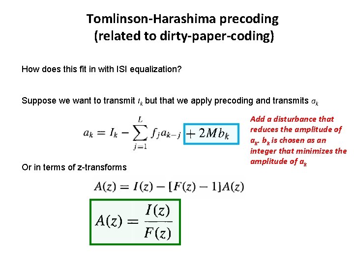
Tomlinson-Harashima precoding (related to dirty-paper-coding) How does this fit in with ISI equalization? Suppose we want to transmit Ik but that we apply precoding and transmits ak Or in terms of z-transforms Add a disturbance that reduces the amplitude of ak. bk is chosen as an integer that minimizes the amplitude of ak

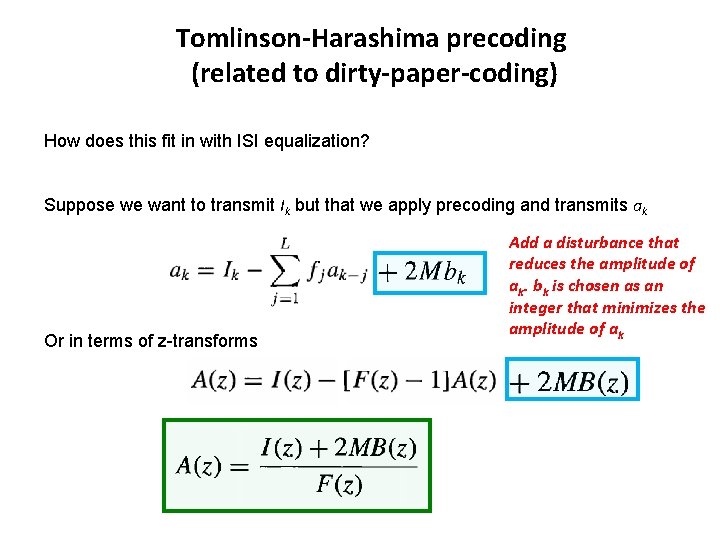
Tomlinson-Harashima precoding (related to dirty-paper-coding) How does this fit in with ISI equalization? Suppose we want to transmit Ik but that we apply precoding and transmits ak Or in terms of z-transforms Add a disturbance that reduces the amplitude of ak. bk is chosen as an integer that minimizes the amplitude of ak

Tomlinson-Harashima precoding (related to dirty-paper-coding) How does this fit in with ISI equalization? Suppose we want to transmit Ik but that we apply precoding and transmits ak Or in terms of z-transforms Add a disturbance that reduces the amplitude of ak. bk is chosen as an integer that minimizes the amplitude of ak Channel ”removes” F(z), modulus operation ”removes” 2 MB(z)

Chapter 10

Objectives • So far, we only considered the case where the channel fn was known in advance • Now we consider the case when the channel is unknown, but a training block of known data symbols are present • We aim at establishing low-complexity adaptive methods for finding the optimal equalizer filters • This chapter has many applications outside of digital communications

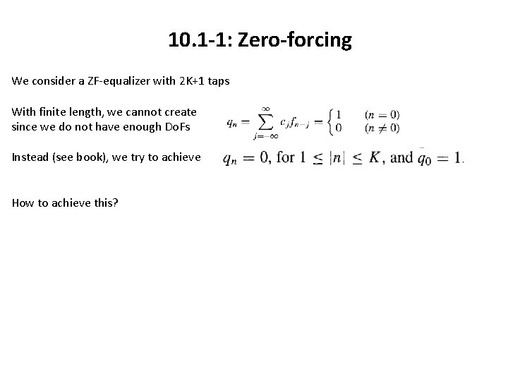
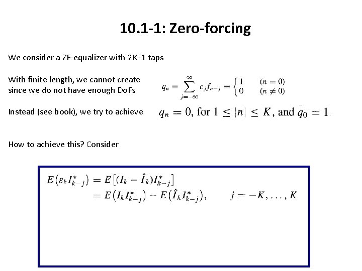
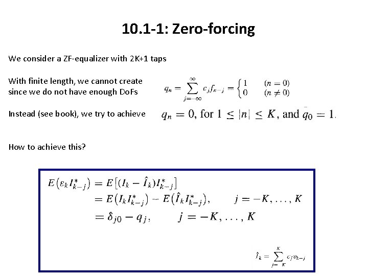
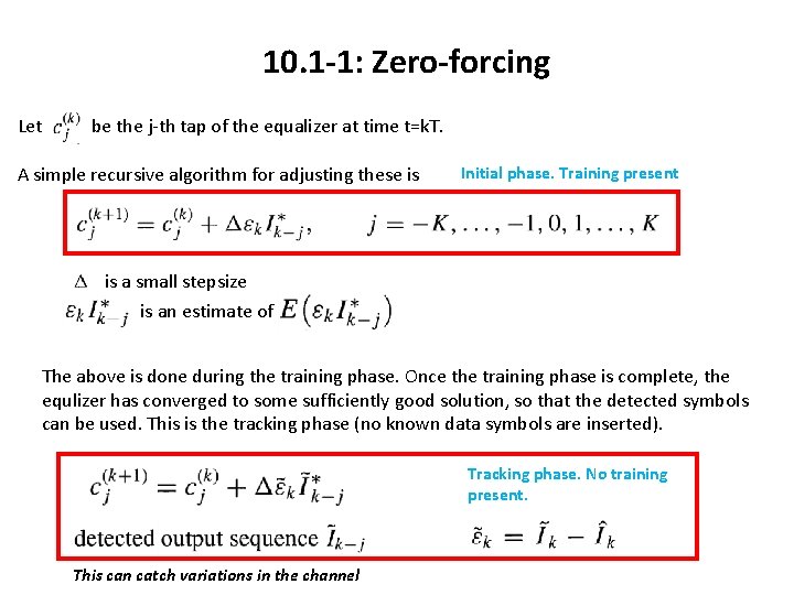
10. 1 -1: Zero-forcing We consider a ZF-equalizer with 2 K+1 taps With finite length, we cannot create since we do not have enough Do. Fs Instead (see book), we try to achieve How to achieve this?

10. 1 -1: Zero-forcing We consider a ZF-equalizer with 2 K+1 taps With finite length, we cannot create since we do not have enough Do. Fs Instead (see book), we try to achieve How to achieve this? Consider

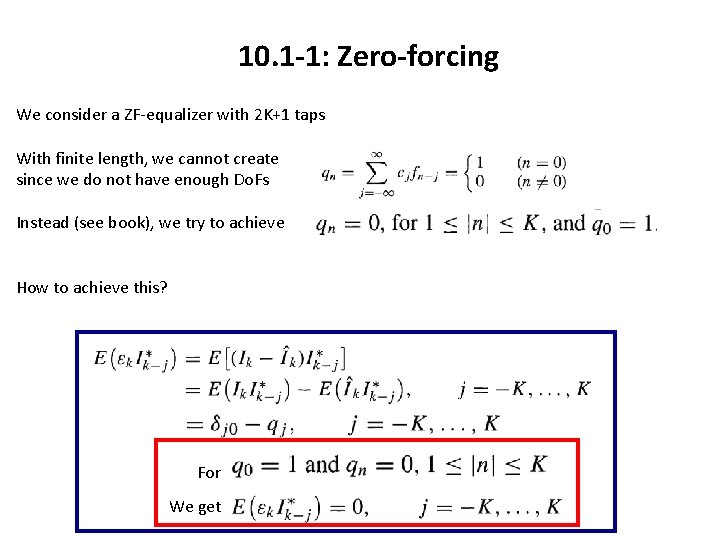
10. 1 -1: Zero-forcing We consider a ZF-equalizer with 2 K+1 taps With finite length, we cannot create since we do not have enough Do. Fs Instead (see book), we try to achieve How to achieve this?

10. 1 -1: Zero-forcing We consider a ZF-equalizer with 2 K+1 taps With finite length, we cannot create since we do not have enough Do. Fs Instead (see book), we try to achieve How to achieve this? For We get

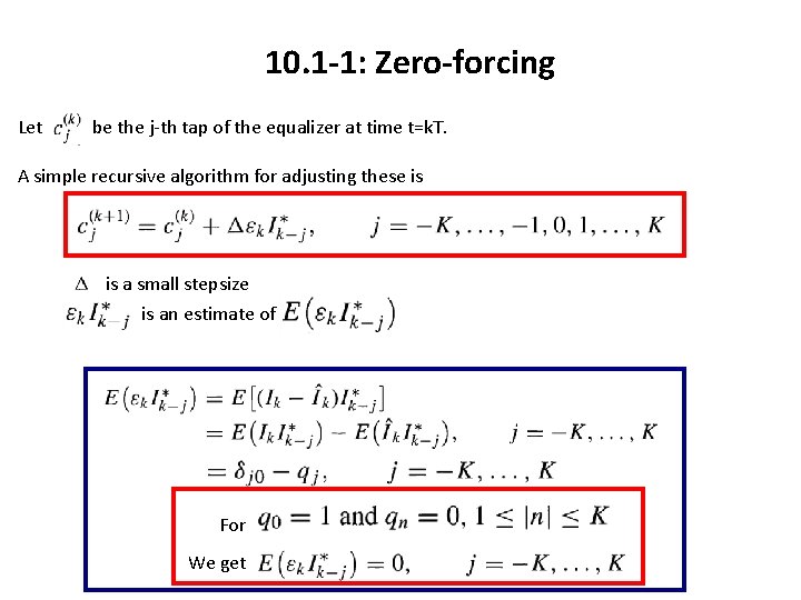
10. 1 -1: Zero-forcing Let be the j-th tap of the equalizer at time t=k. T. A simple recursive algorithm for adjusting these is a small stepsize is an estimate of For We get

10. 1 -1: Zero-forcing Let be the j-th tap of the equalizer at time t=k. T. A simple recursive algorithm for adjusting these is Initial phase. Training present is a small stepsize is an estimate of The above is done during the training phase. Once the training phase is complete, the equlizer has converged to some sufficiently good solution, so that the detected symbols can be used. This is the tracking phase (no known data symbols are inserted). Tracking phase. No training present. This can catch variations in the channel

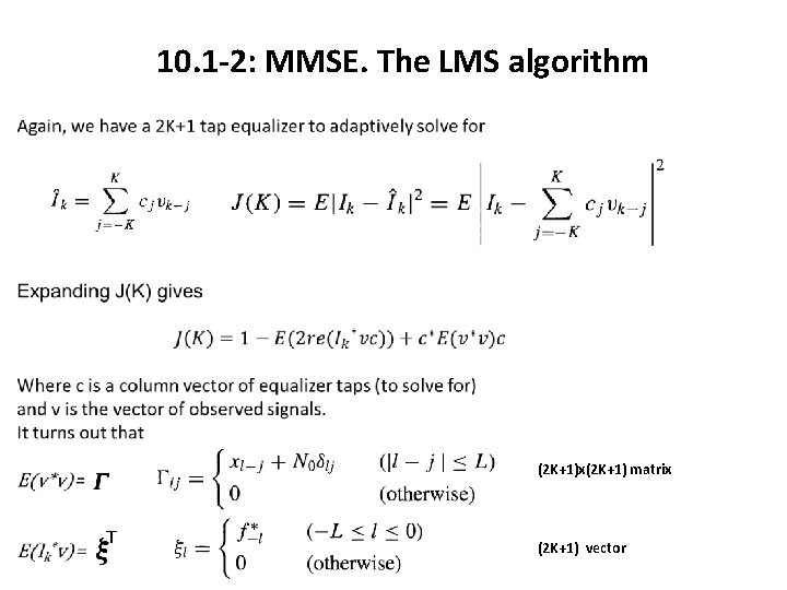
10. 1 -2: MMSE. The LMS algorithm (2 K+1)x(2 K+1) matrix T (2 K+1) vector

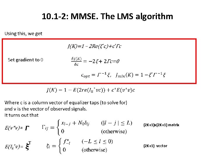
10. 1 -2: MMSE. The LMS algorithm Set gradient to 0 (2 K+1)x(2 K+1) matrix T (2 K+1) vector

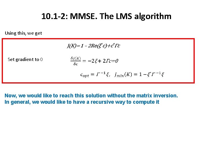
10. 1 -2: MMSE. The LMS algorithm Using this, we get J(K)=1 – 2 Re(ξ*c)+c*Γc Set gradient to 0 Now, we would like to reach this solution without the matrix inversion. In general, we would like to have a recursive way to compute it

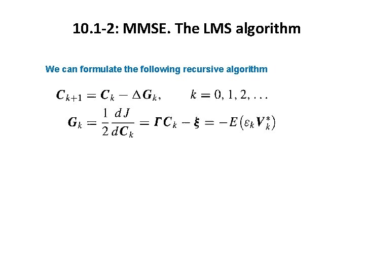
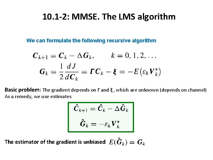
10. 1 -2: MMSE. The LMS algorithm We can formulate the following recursive algorithm

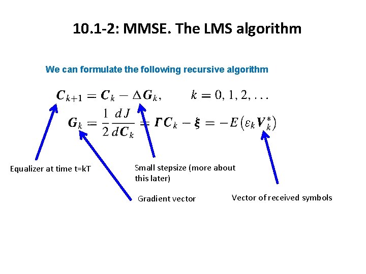
10. 1 -2: MMSE. The LMS algorithm We can formulate the following recursive algorithm Equalizer at time t=k. T Small stepsize (more about this later) Gradient vector Vector of received symbols

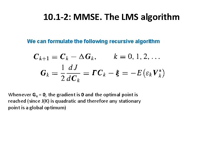
10. 1 -2: MMSE. The LMS algorithm We can formulate the following recursive algorithm Whenever Gk = 0, the gradient is 0 and the optimal point is reached (since J(K) is quadratic and therefore any stationary point is a global optimum)

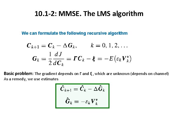
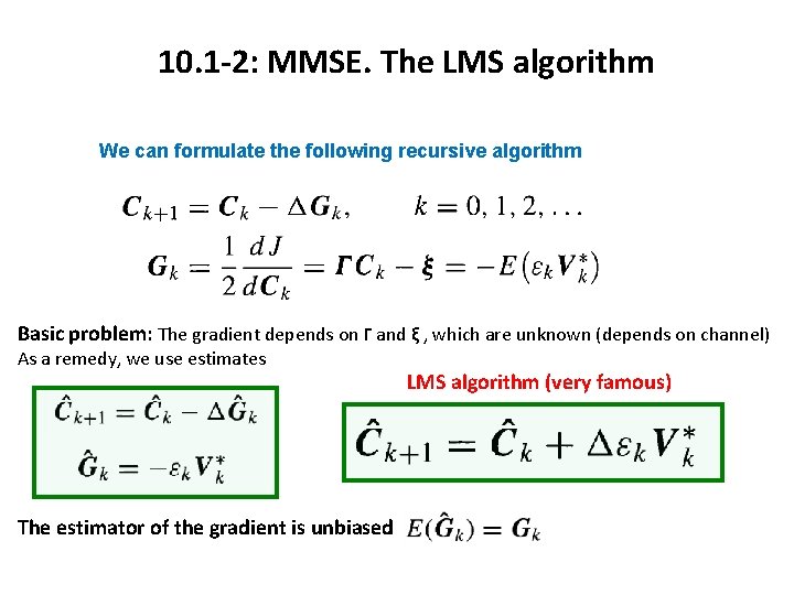
10. 1 -2: MMSE. The LMS algorithm We can formulate the following recursive algorithm Basic problem: The gradient depends on Γ and ξ , which are unknown (depends on channel) As a remedy, we use estimates

10. 1 -2: MMSE. The LMS algorithm We can formulate the following recursive algorithm Basic problem: The gradient depends on Γ and ξ , which are unknown (depends on channel) As a remedy, we use estimates The estimator of the gradient is unbiased

10. 1 -2: MMSE. The LMS algorithm We can formulate the following recursive algorithm Basic problem: The gradient depends on Γ and ξ , which are unknown (depends on channel) As a remedy, we use estimates The estimator of the gradient is unbiased LMS algorithm (very famous)

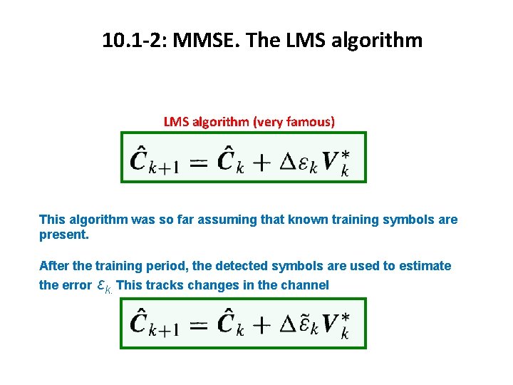
10. 1 -2: MMSE. The LMS algorithm (very famous) This algorithm was so far assuming that known training symbols are present. After the training period, the detected symbols are used to estimate the error εk. This tracks changes in the channel

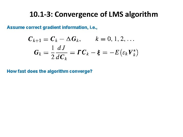
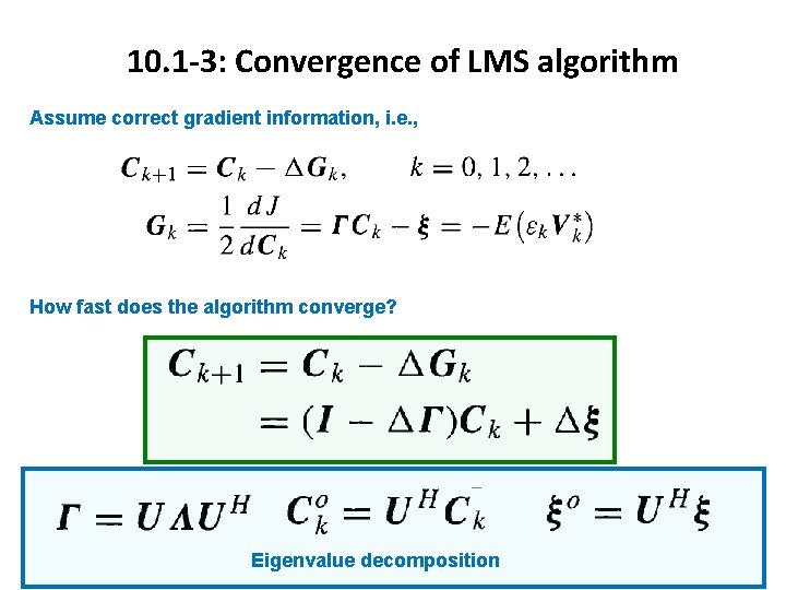
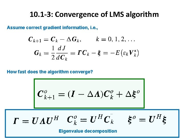
10. 1 -3: Convergence of LMS algorithm Assume correct gradient information, i. e. , How fast does the algorithm converge?

10. 1 -3: Convergence of LMS algorithm Assume correct gradient information, i. e. , How fast does the algorithm converge? Eigenvalue decomposition

10. 1 -3: Convergence of LMS algorithm Assume correct gradient information, i. e. , How fast does the algorithm converge? Eigenvalue decomposition

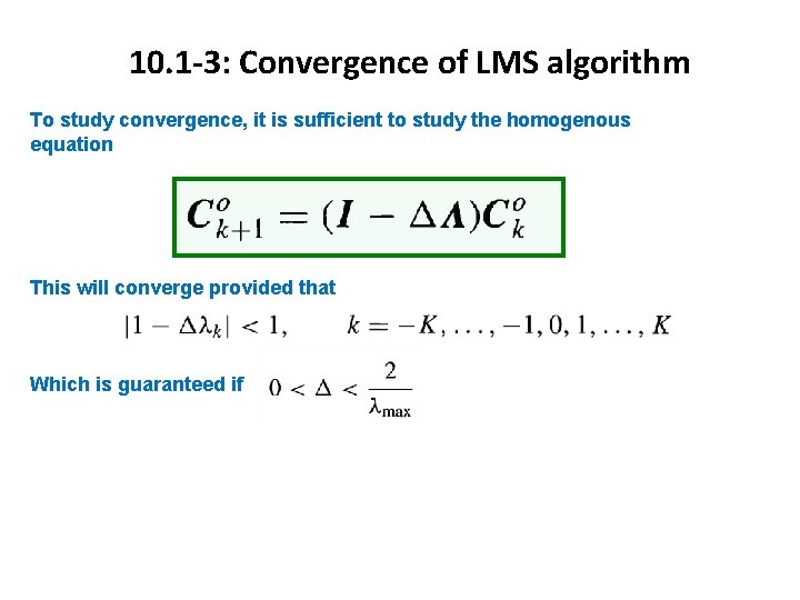
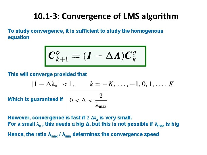
10. 1 -3: Convergence of LMS algorithm To study convergence, it is sufficient to study the homogenous equation This will converge provided that Which is guaranteed if

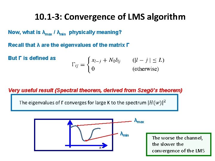
10. 1 -3: Convergence of LMS algorithm To study convergence, it is sufficient to study the homogenous equation This will converge provided that Which is guaranteed if However, convergence is fast if 1 -Δλk is very small. For a small λk , this needs a big Δ, but this is not possible if λmax is big Hence, the ratio λmax / λmin determines the convergence speed

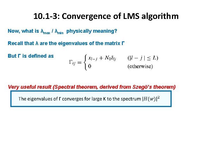
10. 1 -3: Convergence of LMS algorithm Now, what is λmax / λmin physically meaning? Recall that λ are the eigenvalues of the matrix Γ But Γ is defined as Very useful result (Spectral theorem, derived from Szegö’s theorem)

10. 1 -3: Convergence of LMS algorithm Now, what is λmax / λmin physically meaning? Recall that λ are the eigenvalues of the matrix Γ But Γ is defined as Very useful result (Spectral theorem, derived from Szegö’s theorem) λmax λmin π The worse the channel, the slower the convergence of the LMS

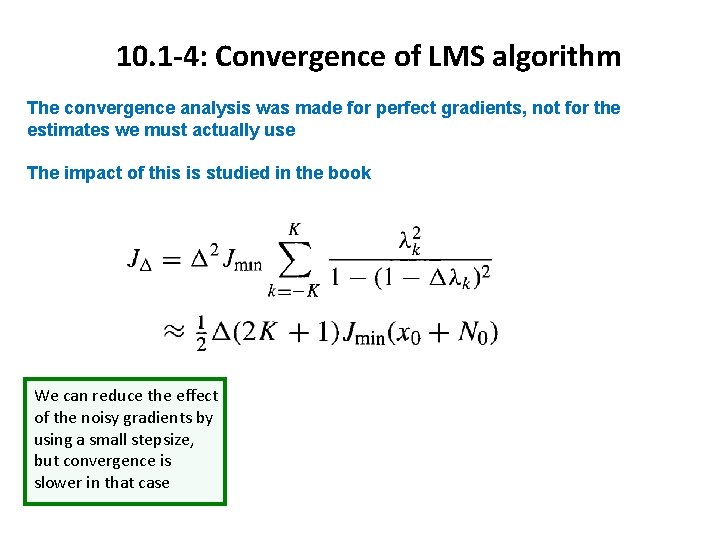
10. 1 -4: Convergence of LMS algorithm The convergence analysis was made for perfect gradients, not for the estimates we must actually use The impact of this is studied in the book We can reduce the effect of the noisy gradients by using a small stepsize, but convergence is slower in that case

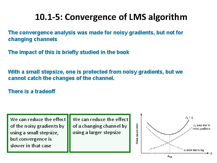
10. 1 -5: Convergence of LMS algorithm The convergence analysis was made for noisy gradients, but not for changing channels The impact of this is briefly studied in the book With a small stepsize, one is protected from noisy gradients, but we cannot catch the changes of the channel. There is a tradeoff We can reduce the effect of the noisy gradients by using a small stepsize, but convergence is slower in that case We can reduce the effect of a changing channel by using a larger stepsize

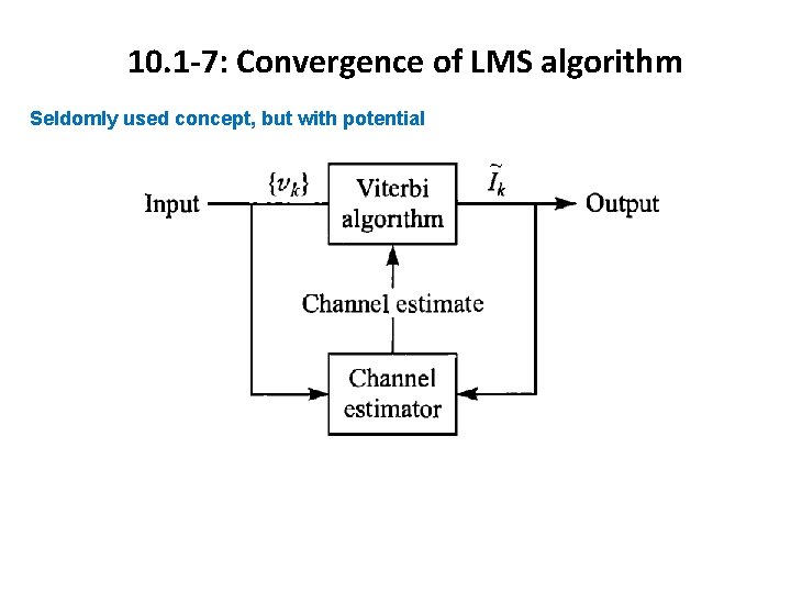
10. 1 -7: Convergence of LMS algorithm Seldomly used concept, but with potential

Section 10. 4. RLS algorithm (Kalman) The problem of LMS is that there is only a single design parameter, namely the stepsize. Still, we have 2 K+1 taps to optimize RLS leverages this and uses 2 K+1 design parameters. Convergence is extremely fast, at the price of high computational complexity

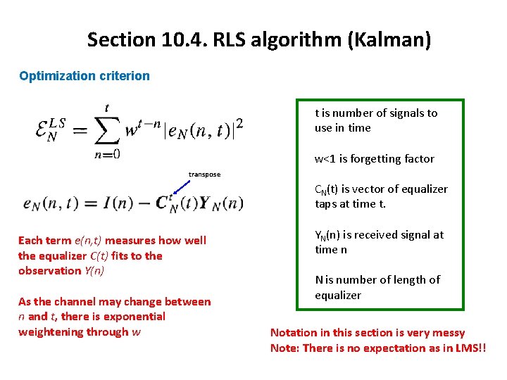
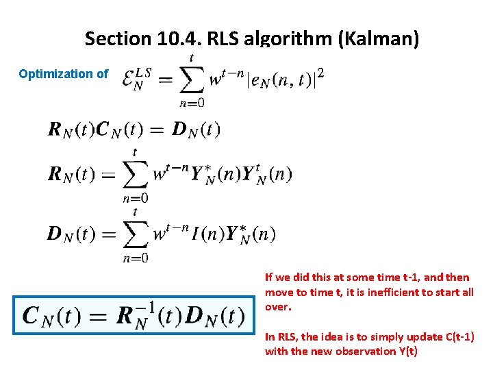
Section 10. 4. RLS algorithm (Kalman) Optimization criterion t is number of signals to use in time w<1 is forgetting factor transpose CN(t) is vector of equalizer taps at time t. Each term e(n, t) measures how well the equalizer C(t) fits to the observation Y(n) As the channel may change between n and t, there is exponential weightening through w YN(n) is received signal at time n N is number of length of equalizer Notation in this section is very messy Note: There is no expectation as in LMS!!

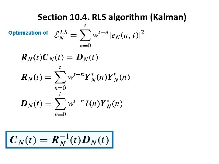
Section 10. 4. RLS algorithm (Kalman) Optimization of

Section 10. 4. RLS algorithm (Kalman) Optimization of If we did this at some time t-1, and then move to time t, it is inefficient to start all over. In RLS, the idea is to simply update C(t-1) with the new observation Y(t)

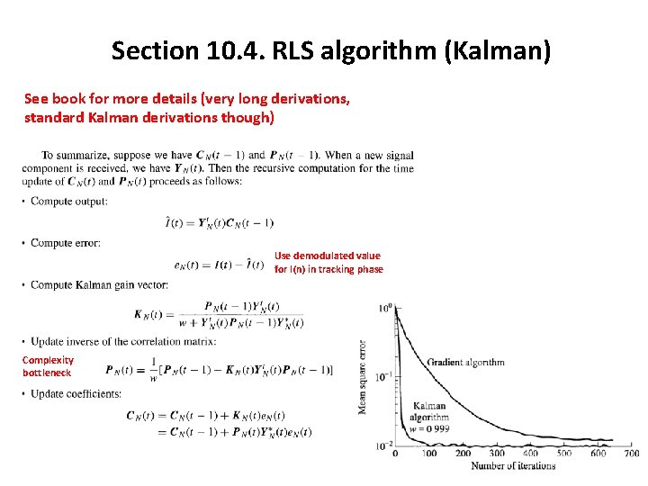
Section 10. 4. RLS algorithm (Kalman) See book for more details (very long derivations, standard Kalman derivations though) Use demodulated value for I(n) in tracking phase Complexity bottleneck

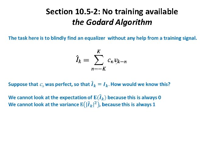
Section 10. 5 -2: No training available the Godard Algorithm

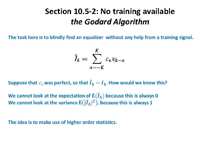
Section 10. 5 -2: No training available the Godard Algorithm

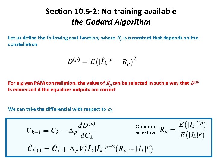
Section 10. 5 -2: No training available the Godard Algorithm Let us define the following cost function, where Rp is a constant that depends on the constellation For a given PAM constellation, the value of Rp can be selected in such a way that D(p) Is minimized if the equalizer outputs are correct We can take the differential with respect to ck Optimum selection

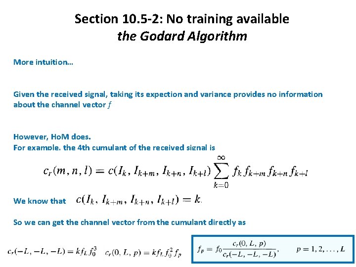
Section 10. 5 -2: No training available the Godard Algorithm More intuition… Given the received signal, taking its expection and variance provides no information about the channel vector f However, Ho. M does. For example, the 4 th cumulant of the received signal is We know that So we can get the channel vector from the cumulant directly as