DIAGRAMMATIC MONTE CARLO N Prokofev Kourovka 2018 Advancing

DIAGRAMMATIC MONTE CARLO: N. Prokof’ev Kourovka, 2018 Advancing Research in Basic Science and Mathematics

Complexity of an interacting fermion problem Ask the relevant physical question “What does it take to obtain some quantity A with accuracy ? ” in thermodynamic limit (TL) [macroscopically large system] Think of experiment! 1. Without specifying a particular method of getting A , it makes no sense to talk about fermioninc sign problem. 2. Theoretically, we need to define the computational The method is said to have CCP if the CPU time, faster than any polynomial function of Why thermodynamic limit? In a system with complexity problem (CCP) as , required to compute with accuracy . The problem is considered solved if particles the ultimate scaling is always central-limit theorem (if this scaling can be reached in practice; say for ) diverges. by the

Sing Problem for methods based on Z when is not always positive with If we do not know the answer even approximately If we can live that long and then accuracy is , but we need Ultimately, accuracy is limited by finite-size corrections that can remain too large in some cases. Compromise: systematic bias (variational, AFQMC, …)

Simple observation Let is a convergent series with convergence radius . Define finite sums: Then , is such that Even if it takes with , to compute , the computation time required to obtain with any specified relative accuracy is subject to polynomial scaling CCP is solved! When accuracy gain is exponential in one should not consider exponential scaling as a problem preventing us from computing A with high (and systematically improvable) accuracy

Diag. MC for connected Feynman diagrams vs CCP for fermions explicitly in thermodynamic limit (connected diagrams) Sign-blessing I: Feynman diagrammatic expansions converge only if same order diagrams cancel each other (for lattice fermions at finite T) Sign-blessing II: Sum of all connected topologies carry some properties of fermionic determinants (sums of all connected and disconnected graphs; n! terms in n 3 operations) For convergent series with For fermions, all order-N connected graphs can be computed in time [R. Rossi, PRL ‘ 17] CCP is solved by Diag. MC:

Personal viewpoint (at least at the level of standard thermodynamics): If it can be measured experimentally it can be calculated theoretically on classical computers with the same accuracy … we just don’t know yet how exactly in many cases …

Bold (self-consistent) Diagrammatic Monte Carlo Diagrammatic technique for ln(Z ) diagrams: admits partial summation and self-consistent formulation No need to compute all diagrams for and : Dyson Equation: Screening: Calculate irreducible diagrams for , , … to get , , …. from Dyson equations

One possible scheme: G 2 W- expansion . . . . In terms of “exact” propagators Dyson Equation: Screening: .

More tools: Build diagrams using ladders: (contact potential) In terms of “exact” propagators Dyson Equations:

More tools: Build diagrams using three ladders: (contact potential) The only triple-couting (at the lowest order)

Fully dressed skeleton graphs (Heidin): . Irreducible 3 -point vertex: all accounted for already! .

Bare or “dressed” series or skeleton sequences? Pros. for bare: - Taylor series theory of analytic functions & resummation techniques [work outside of convergence radius] - in diagrams are analytic; no self-consistent loops Pros. for dressed/skeleton: - Same graphs as in bare, just a much smaller set # of irreducible graphs at order n is smaller by a factor of about 1/n for each “dressed” channel: , One can simulate higher orders faster - are readily available from tables as fast and easy, as intrinsic - Bare series for long-range interactions are ill-defined, e. g. for the 2 d-order bubble diagram involves. Need to screen, or sum up all bubble chains.

Pros. for dressed/skeleton: - Different expansion parameter: consider a dilute gas with large V. Define a pair propagator based on ladder diagrams, and arrive at the techniques where expension is in powers of density, not V. Con. for skeleton: - Skeleton sequence for divergent bare series may converge to the wrong answer! Solution for this Con. - dress lines only partially by low-order bare or skeleton graphs - do Taylor series for the rest using an auxiliary parameter

Shifted action tools Original setup: Bare series produce Taylor series in and the physical answer corresponds to Introduce Unphysical, in general, with formally arbitrary set of functions , but if we demand then at we will recover the physical action identically . Proceed with Taylor series expansion in but it’s a different series because of counter-terms - If are based on diagrams, then we expand on top of partially dressed G - If are based on diagrams, then we deal with skeleton dressing - This setup can be generalized (with the help of Hubbard-Stratanovich transformation) to partial or skeleton dressing of interactions, ladders, etc.

When series diverge or convergence is slow Recall Complex plane pole branch cut This is just a cartoon analogy, in shifted action we change the “origin of expansion” in the functional space, and =0 may not be even physical

When series diverge or convergence is slow Complex U plane Complex z plane Conformal mapping: Generalization = Pade Hypergeometric functions Borel, conformal Borel, never-heard-of-method …

When convergence radius is zero & series are asymptotic (unitary ultra-cold Fermi gas) Quantitative understanding of series divergent behavior saddle-point in g method for large exp. saddle-point in g and bosonic field (after Hubbard-Stratanovich transformation) for large exponent L. N. Lipatov, Sov. Phys. JETP 45, 216 (1977)] - Can be generalized for partially summed and skeleton series - Suggests efficient resummation technique & uniqueness of Z(g) - “designer” conformal Borel transforms series from asymptotic to convergent! R. Rossi, K. van Houcke, F. Werner ‘yesterday

If you can - compute enough orders (say n~10; billions of skeleton graphs) and - know what to do with them, then any interacting Fermi system can be solved accurately

Sign alternating statistics Sample or sum? (Diagrammatic series for fermions converge, despite having about n! of them at order n, only because they cancel each other ) Sample Sum exact answer ! Definitely sum!

Spending CPU on performing “smart” global updates Let with , then making local updates is not optimal because getting an uncorrelated set will require updates ``Learn’’ how propose global updates with accaptance ratio . ``Heat bath’’ idea + ``self-learning’’ algoritms Type A updates: Interpret the second ratio as the relative weight of configurations when proposing a change.

Monte Carlo Markov-chain cycle: Accept/Reject propose Accept/Reject Local update … Large number L >> n of fast local updates One of the ways to make a multi-dimensional stochastic proposal, one variable at a time. If and is simple enough, then the CPU cost is close to none! The only thing left is to optimize Within some variational ansatz for “Learn” your to be such that minimize on trial runs (or at least >>1/n )

Never did it myself yet (or know of any data for connected Feynman graphs), so … In real space one may try to measure the gyration radius where is the graph’s “center of mass”, and measure the asymptotic dependence when One possible form is Within the Rg ball control Dipole, quadrupole, etc. fluct.

Applications: “Yes, we can, but …”

- Free energy density When series converge: 2 D Fermi-Hubbard model at R. Rossi, PRL ‘ 17 Six to five digit (depending on quantity) accuracy for a finite-T answer!

When series converge Fermi-liquid @ T-independent in Fermi-liquid

Conclusions/perspectives we Fo n r U SI ee M > M O AN N d a 4 d. an Y S C EL OL iff d EC LA ere. n TR BO nt >0 s. 7 O R N AT ch em PR I O O N e B LE ON M Any dispersion relation for the same U and n

What did we know with meaningful error bars FM ? ? Stripes ? ? AFM ? ? PHASE SEPARATION? ? ?

Cooper instability in the BCS regime is temperature (and frequency) independent in the limit Fermi-liquid form at determines

Protocol: Compute Fermi surface parameters ; verify their T-independence Transform Solve for eigenvectors and eigenfunctions Predicted divergence (standard weak-coupling BCS) To determine compute correction (future work): is -independent, to leading order in small g

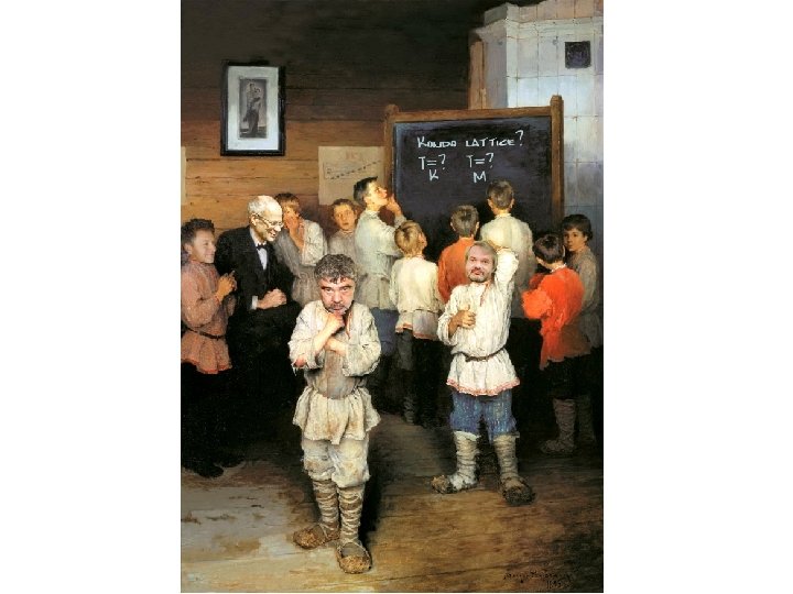
Hlubina, PRB 59, 9600 (1999) up to

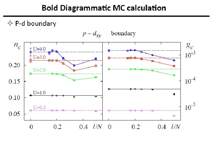
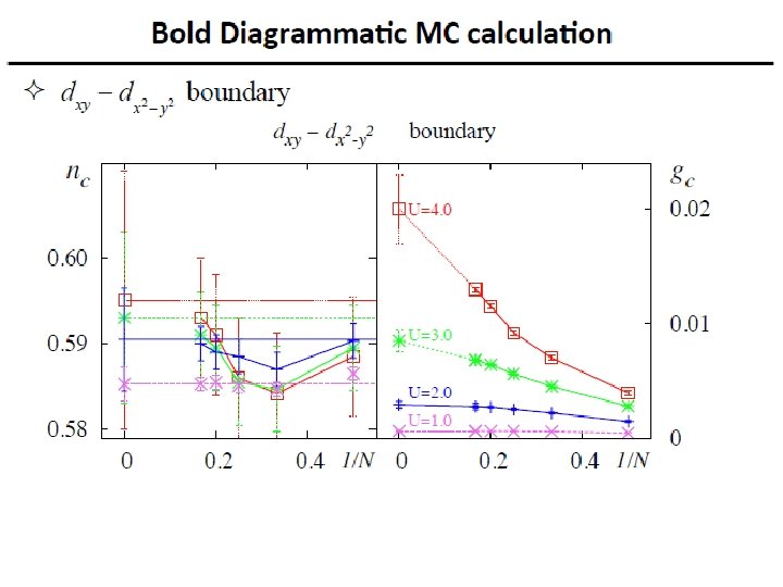
BOLD DIAGRAMMATIC CALCULATION: G&T-matrix self-consistent skeleton formulation (contact potential) Define “bare” pair propagator : (exact solution of the two-body problem) Skeleton diagrams In terms of “exact” or “fully dressed” propagators & Dyson Equations:

BOLD DIAGRAMMATIC CALCULATION: G&T-matrix self-consistent formulation (contact potential)

When series converge Dispersion relation Graphene-type system Dirac points (dimensionless coupling) in suspended graphene An the “roller-coaster” story goes as …

Fock diagram Gonzalez, Guinea, and. Vozmediano ‘ 94 In RG language using renormalized dispersion or asymptotically free Dirac liquid Adding next order diagrams Mishchenko ‘ 07; Vafek and Case ‘ 08 Possibility of an unstable fixed point at Dirac liquid insuator

But the value of is not small and the answer cannot be trusted! Gonza´lez, Guinea, and Vozmediano ‘ 99; Das Sarma, Hwang, and Tse ‘ 07; Polini et al. ‘ 07; Son ‘ 07; Foster and Aleiner ‘ 08; Kotov, Uchoa, and Castro Neto ‘ 09 Upgrading 2 d-order calculation to RPA: From to = + + +… sreened int. is now such that Dirac liquid is back! (by adding some but not all graphs) But for the answer cannot be trusted either!

Direct numerical simulation: Hybrid Deperminant Quantum Monte Carlo (no sign-problem in the particle/hole symmetric case; L/a=24) Coulomb law after on-site U Hands and Strouthos ‘ 08 Drut and La¨hde ’ 09 Dirac liquid insulator for But … experiments find Dirac liquid in suspended graphene! Fermi velocity (density dependence) Elias, Gorbachev, Mayorov, Morozov, Zhukov, Blake, Ponomarenko, Grigorieva, Novoselov, Guinea, Geim, Mukhin ’ 11 -’ 12 ARPES Siegel, Park, Hwang, Deslippe, Fedorov, Louie, and Lanzara, ‘ 11

Hybrid Deperminant Quantum Monte Carlo Ulybyshev, Buividovich, Katsnelson, and Polikarpov ’ 12 -’ 13 Smith and von Smekal ‘ 14). Dirac liquid in suspended graphene is back alive! Status of previous work Short-range correlations are extremely important in graphene; they prevent one from revealing the long-range Coulomb effects in finite systems. No solution for RG flow of (beyond uv RG cutoff scale)

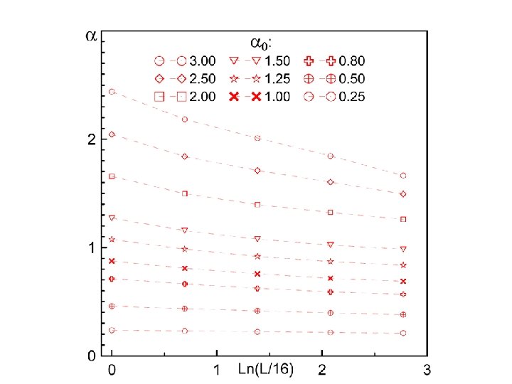
BDMC approach 1. Eliminate Mott-insulator instability by making potential Flat! flat at short-range can study larger values of 2. We can afford electrons with and RG flow up to L=256 (a) The flow is always to weaker coupling (b) changes are small

Flowgram idea Kuklov, Matsumoto, NP, Svistunov, Troyer ‘ 08 Single parameter flow assumption/universality (at large distances) : with universal flow functions All dependence on microscopic parameters is in or If for two systems A and B we get then the flows for and should be the same. In terms of selecting a different value of is equivalent to a horizontal shift If true, expect data collapse and a smooth “master” curve; if false, observe derivative jumps

Match and obtain a smooth RG flow curve spanning 15 orders of magnitude! (from simulations of 14 different microscopic Hamiltonians) Finally, increase the maximum diagram order in the skeleton expansion to account for vertex corrections. Dirac liquid in a graphene-type system is stable against strong Coulomb interaction

E. g. quantum Heisenberg model Popov-Fedotov trick Two-body spin-dependent interaction with complex Standard diagrammatic technique (with “flat-band” bare dispersion) Compute diagram after diagram for, say, proper self-energy and polarization … Reliable results down to temperature T=J/6 for pyrochlore lattice

Heisenberg model on pyrochlore lattice (3 D Kagome) Cooperative paramagnet Ising spin-ice ? Emergent ? spin-ice ? How the SU(2) cooperative paramagnet looks like? ____ ? U(1) spin liquid Y. Huang, K. Chen, Y. Deng, NP, and B. Svistunov ‘ 16

+ Classical-to-Quantum correspondence ---“fingerprint” identification of quantum states) Let . Then for any there exists such that for any distance R

Classical-to-Quantum correspondence is accurate at the level of 0. 3% (but not exact)

When series diverge or convergence is slow: 2 D Fermi-Hubbard model (optimize for best convergence in the atomic limit) Divergent series Expansion order W. Wu, M. Ferrero, A. Georges, E. Kozik,

When series diverge or convergence is slow: 2 D Fermi-Hubbard model Use to study pseudogap physics at Nodal vs anti-nodal dichotomy. What scattering processes dominate at different parts of FS?

When series diverge or convergence is slow Solution of the non-equilibrium transport through Kondo impurity

When the convergence radius is zero: unitary Fermi gas Fermions with strong “zero”-range potential leading to large s-wave scattering length Unitary limit: In this case and are the only length/energy scales Skeleton diagrammatic series are asymptotic with leading divergence , but are subject to the series resummation technique

Real thing, not a cartoon! tiny 10 -6 fraction

Equation of state for the unitary Fermi gas (superfluid transition is at R. Rossi, F. Werner, K. van Houcke (private comm. ‘ 16)

Conclusions: 1. For convergent and subject to re-summation series, Diag. MC solves the computational complexity problem ( ) correlated fermionic systems can be addressed with systematically improvable accuracy. What we lack is theoretical understanding of analytic properties of the model properties. 2. If item 1 above is understood, then the possibilities are unlimited ! - Hubbard model (need better formulations near half-filling -> second fermionization, dual fermions, parquet, … - Resonant fermions (develop Diag. MC for superfluid states, explore polarized gases, move away from unitarity, …) - frustrated magnets (unique method for the cooperative paramagnet regime (can do pyrochlore), but need to explore alternative formulations for T<<J, develop SU(N) schemes, …) - interacting topological materials (ready to explore stability bounds and phase diagrams) - Real materials? In progress (Simons Collaboration on the Many Electron Problem)

imaginary time + + Lattice path-integrals for particles and spins are “diagrams” of closed loops formed by occupation number trajectories

+ Diagrams for imaginary time Diagrams for lattice site The rest is conventional worm algorithm in continuous time

Find the. . . differences Simulations can handle up to particles at exper. relevant temperature

No fit comparison of timeof-flight images (momentum distributions) S. Trotzky, L. Pollet, F. Gerbier, U. Schnorrberger, I. Bloch, NP B. Svistunov, M. Troyer, ‘ 10

Path-integrals in continuous space are “diagrams” of closed loops too! P 2 1 P

Diagrams for the attractive tail in : If and N>>1 all the effort is for something small ! P statistical interpretation 2 1 ignore : stat. weight 1 Account for : stat. weight p P Faster than conventional scheme for N>30, scalable (size independent) updates with exact account of interactions between all particles

3 D @ s. v. p. 64 experiment 2048

Diagrammatic expansions Positive-definite Any math. representation of the problem Sign-blessed Polarons Connected diagrams Diag. MC (for bare series expansions) Rossi ar. Xiv: 1612. 05184 Path integrals for bosins/spins Sign-blessed Positive-definite Continuous time (CT) Determinant Diag. MC Impurity solvers, …

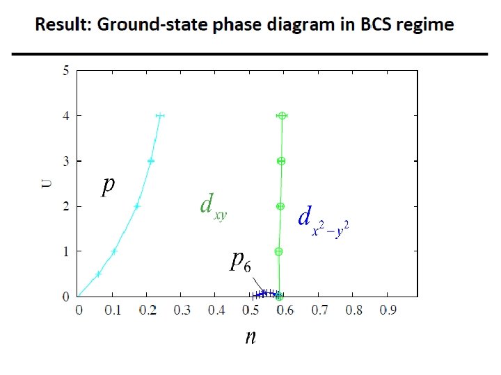
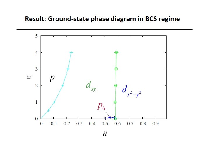
p-pairing dominates only d-pairing

Compensation trick: Original representation Identical representation (under integration) Arbitrary auxiliary function with “Design” it to compensate