Deep Networks Jianping Fan CS Dept UNCCharlotte Deep

Deep Networks Jianping Fan CS Dept UNC-Charlotte

Deep Networks 1. Alex. Net 2. VGG 3. Google. Net 4. Res. Net

Some Pri-knowledge for Deep Networks Perceptron

Multi-layer perceptron

Sigmoid function

Artificial Neural Network 3 -layer

Handwriting Recognition

Digit Recognition NN 24 x 24 = 784 0. 0 white 1. 0 black

Convolutional Neural Networks: Alex. Net Lion Image labels Krizhevsky, Sutskever, Hinton — NIPS 2012

Layer 1 Filter (Gabor and color blobs) Layer 2 Layer 5 Last Layer Zeiler et al. ar. Xiv 2013, ECCV 2014 Gabor filter: linear filters used for edge detection with similar orientation representations to the human visual system Nguyen et al. ar. Xiv 2014

Alex. Net conv max pool. . . conv max pool. . .

Alex. Net . . . FC FC Softmax 1000 4096

Convolutional Neural Network • 3 main types of layers • Convolutional layer • Pooling layer • Fully Connected layer

Activation function

Convolutional Neural Network

Example of CNN layer

Convolutional layer

96 filters of 11 x 3 each

Pooling or downsampling

Receptive Field conv

Input 3 x 3 conv, 64 Pool 3 x 3 conv, 128 Pool 3 x 3 conv, 256 Pool 3 x 3 conv, 512 3 x 3 conv, 512 Pool FC 4096 FC 1000 memory: memory: memory: memory: memory: memory: 224*3=150 K params: 0 224*64=3. 2 M params: (3*3*3)*64 = 1, 728 224*64=3. 2 M params: (3*3*64)*64 = 36, 864 112*64=800 K params: 0 112*128=1. 6 M params: (3*3*64)*128 = 73, 728 112*128=1. 6 M params: (3*3*128)*128 = 147, 456 56*56*128=400 K params: 0 56*56*256=800 K params: (3*3*128)*256 = 294, 912 56*56*256=800 K params: (3*3*256)*256 = 589, 824 28*28*256=200 K params: 0 28*28*512=400 K params: (3*3*256)*512 = 1, 179, 648 28*28*512=400 K params: (3*3*512)*512 = 2, 359, 296 14*14*512=100 K params: 0 14*14*512=100 K params: (3*3*512)*512 = 2, 359, 296 7*7*512=25 K params: 0 4096 params: 7*7*512*4096 = 102, 760, 448 4096 params: 4096*4096 = 16, 777, 216 1000 params: 4096*1000 = 4, 096, 000

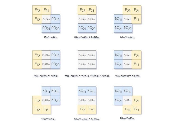
Backpropagation of convolution

To calculate the gradients of error ‘E’ with respect to the filter ‘F’, the following equations needs to solved.

Which evaluates to-

If we look closely the previous equation can be written in form of our convolution operation.

Similarly we can find the gradients of the error ‘E’ with respect to the input matrix ‘X’.

The previous computation can be obtained by a different type of convolution operation known as full convolution. In order to obtain the gradients of the input matrix we need to rotate the filter by 180 degree and calculate the full convolution of the rotated filter by the gradients of the output with respect to error. F 11 F 12 F 21 F 22 Rotate x F 12 F 11 F 22 F 21 Rotate y F 22 F 21 F 12 F 11

Backpropagation of max pooling Suppose you have a matrix M of four elements: a c b d and maxpool(M) returns d. Then, the maxpool function really only depends on d. So, the derivative of maxpool relative to d is 1, and its derivative relative to a, b, c is zero. So you backpropagate 1 to the unit corresponding to d, and you backpropagate zero for the other units.

VGGNet • Very Deep Convolutional Networks For Large Scale Image Recognition - Karen Simonyan and Andrew Zisserman; 2015 • The runner-up at the ILSVRC 2014 competition • Significantly deeper than Alex. Net • 140 million parameters

Input 3 x 3 conv, 64 Pool 1/2 3 x 3 conv, 128 Pool 1/2 3 x 3 conv, 256 Pool 1/2 3 x 3 conv, 512 3 x 3 conv, 512 Pool 1/2 FC 4096 FC 1000 Softmax VGGNet • Smaller filters Only 3 x 3 CONV filters, stride 1, pad 1 and 2 x 2 MAX POOL , stride 2 • Deeper network Alex. Net: 8 layers VGGNet: 16 - 19 layers • ZFNet: 11. 7% top 5 error in ILSVRC’ 13 • VGGNet: 7. 3% top 5 error in ILSVRC’ 14

VGGNet • Why use smaller filters? (3 x 3 conv) Stack of three 3 x 3 conv (stride 1) layers has the same effective receptive field as one 7 x 7 conv layer. • What is the effective receptive field of three 3 x 3 conv (stride 1) layers? 7 x 7 But deeper, more non-linearities And fewer parameters: 3 * (32 C 2) vs. 72 C 2 for C channels per layer

Input 3 x 3 conv, 64 Pool 3 x 3 conv, 128 Pool 3 x 3 conv, 256 Pool 3 x 3 conv, 512 3 x 3 conv, 512 Pool FC 4096 FC 1000 Softmax VGGNet VGG 16: TOTAL memory: 24 M * 4 bytes ~= 96 MB / image TOTAL params: 138 M parameters

Input 3 x 3 conv, 64 Pool 3 x 3 conv, 128 Pool 3 x 3 conv, 256 Pool 3 x 3 conv, 512 3 x 3 conv, 512 Pool FC 4096 FC 1000 memory: memory: memory: memory: memory: memory: 224*3=150 K params: 0 224*64=3. 2 M params: (3*3*3)*64 = 1, 728 224*64=3. 2 M params: (3*3*64)*64 = 36, 864 112*64=800 K params: 0 112*128=1. 6 M params: (3*3*64)*128 = 73, 728 112*128=1. 6 M params: (3*3*128)*128 = 147, 456 56*56*128=400 K params: 0 56*56*256=800 K params: (3*3*128)*256 = 294, 912 56*56*256=800 K params: (3*3*256)*256 = 589, 824 28*28*256=200 K params: 0 28*28*512=400 K params: (3*3*256)*512 = 1, 179, 648 28*28*512=400 K params: (3*3*512)*512 = 2, 359, 296 14*14*512=100 K params: 0 14*14*512=100 K params: (3*3*512)*512 = 2, 359, 296 7*7*512=25 K params: 0 4096 params: 7*7*512*4096 = 102, 760, 448 4096 params: 4096*4096 = 16, 777, 216 1000 params: 4096*1000 = 4, 096, 000

Google. Net • Going Deeper with Convolutions - Christian Szegedy et al. ; 2015 • • ILSVRC 2014 competition winner Also significantly deeper than Alex. Net x 12 less parameters than Alex. Net Focused on computational efficiency

Google. Net • 22 layers • Efficient “Inception” module - strayed from the general approach of simply stacking conv and pooling layers on top of each other in a sequential structure • No FC layers • Only 5 million parameters! • ILSVRC’ 14 classification winner (6. 7% top 5 error)

Google. Net “Inception module”: design a good local network topology (network within a network) and then stack these modules on top of each other Filter concatenation 1 x 1 convolution 3 x 3 convolution 5 x 5 convolution 1 x 1 convolution 3 x 3 max pooling Previous layer

Google. Net Naïve Inception Model • Apply parallel filter operations on the input : • Multiple receptive field sizes for convolution (1 x 1, 3 x 3, 5 x 5) • Pooling operation (3 x 3) • Concatenate all filter outputs together depth-wise Filter concatenation 1 x 1 convolution 3 x 3 convolution 5 x 5 convolution Previous layer 3 x 3 max pooling

Google. Net • What’s the problem with this? High computational complexity Filter concatenation 1 x 1 convolution 3 x 3 convolution 5 x 5 convolution Previous layer 3 x 3 max pooling

Google. Net Output volume sizes: • 1 x 1 conv, 128: 28 x 128 3 x 3 conv, 192: 28 x 192 5 x 5 conv, 96: 28 x 96 3 x 3 pool: 28 x 256 1 x 1 conv 128 Example: Filter concatenation 3 x 3 conv 192 5 x 5 conv 96 Previous layer 28 x 256 • What is output size after filter concatenation? 28 x(128+192+96+256) = 28 x 672 3 x 3 max pooling

Google. Net • Number of convolution operations: 1 x 1 conv, 128: 28 x 128 x 1 x 1 x 256 3 x 3 conv, 192: 28 x 192 x 3 x 3 x 256 5 x 5 conv, 96: 28 x 96 x 5 x 5 x 256 Total: 854 M ops Filter concatenation 1 x 1 conv 128 3 x 3 conv 192 5 x 5 conv 96 Previous layer 28 x 256 3 x 3 max pooling

Google. Net • Very expensive compute! • Pooling layer also preserves feature depth, which means total depth after concatenation can only grow at every layer. Filter concatenation 1 x 1 conv 128 3 x 3 conv 192 5 x 5 conv 96 Previous layer 28 x 256 3 x 3 max pooling

Google. Net • Solution: “bottleneck” layers that use 1 x 1 convolutions to reduce feature depth (from previous hour). Filter concatenation 1 x 1 convolution 3 x 3 convolution 5 x 5 convolution Previous layer 3 x 3 max pooling

Google. Net • Solution: “bottleneck” layers that use 1 x 1 convolutions to reduce feature depth (from previous hour). Filter concatenation 1 x 1 convolution 3 x 3 convolution 5 x 5 convolution 1 x 1 convolution 3 x 3 max pooling Previous layer

• Number of convolution operations: 1 x 1 conv, 64: 28 x 28 x 64 x 1 x 1 x 256 1 x 1 conv, 128: 28 x 128 x 1 x 1 x 256 3 x 3 conv, 192: 28 x 192 x 3 x 3 x 64 5 x 5 conv, 96: 28 x 96 x 5 x 5 x 264 1 x 1 conv, 64: 28 x 64 x 1 x 1 x 256 Filter Total: 353 M ops concatenation 1 x 1 conv 128 3 x 3 conv 192 5 x 5 conv 96 1 x 1 conv 64 3 x 3 max pooling Previous layer 28 x 256 • Compared to 854 M ops for naive version

Google. Net Details/Retrospectives : • Deeper networks, with computational efficiency • 22 layers • Efficient “Inception” module • No FC layers • 12 x less params than Alex. Net • ILSVRC’ 14 classification winner (6. 7% top 5 error)

Res. Net • Deep Residual Learning for Image Recognition Kaiming He, Xiangyu Zhang, Shaoqing Ren, Jian Sun; 2015 • Extremely deep network – 152 layers • Deeper neural networks are more difficult to train. • Deep networks suffer from vanishing and exploding gradients. • Present a residual learning framework to ease the training of networks that are substantially deeper than those used previously.

Res. Net • ILSVRC’ 15 classification winner (3. 57% top 5 error, humans generally hover around a 5 -10% error rate) Swept all classification and detection competitions in ILSVRC’ 15 and COCO’ 15!

Res. Net • What happens when we continue stacking deeper layers on a convolutional neural network? • 56 -layer model performs worse on both training and test error -> The deeper model performs worse (not caused by overfitting)!

Res. Net • Hypothesis: The problem is an optimization problem. Very deep networks are harder to optimize. • Solution: Use network layers to fit residual mapping instead of directly trying to fit a desired underlying mapping. • We will use skip connections allowing us to take the activation from one layer and feed it into another layer, much deeper into the network. • Use layers to fit residual F(x) = H(x) – x instead of H(x) directly

Res. Net Residual Block Input x goes through conv-relu-conv series and gives us F(x). That result is then added to the original input x. Let’s call that H(x) = F(x) + x. In traditional CNNs, H(x) would just be equal to F(x). So, instead of just computing that transformation (straight from x to F(x)), we’re computing the term that we have to add, F(x), to the input, x.

Res. Net Short cut/ skip connection

Res. Net Full Res. Net architecture: • Stack residual blocks • Every residual block has two 3 x 3 conv layers • Periodically, double # of filters and downsample spatially using stride 2 (in each dimension) • Additional conv layer at the beginning • No FC layers at the end (only FC 1000 to output classes)

Res. Net • Total depths of 34, 50, 101, or 152 layers for Image. Net • For deeper networks (Res. Net-50+), use “bottleneck” layer to improve efficiency (similar to Goog. Le. Net)