Decision Analysis Why is decisionmaking difficult z Too

Decision Analysis

Why is decision-making difficult? z. Too many combinations of options to consider (too much info) z. Consequences of our decisions (payoffs) depend on future events which are not known when decisions have to be made (too little info) SEEM 3530 Decision Analysis I 2

How managers think? “INTUITION” l synergistic thinking l pattern recognition l distillation of experience and well-learnt behaviour l cognitive skills (Isenberg, 1988) SEEM 3530 Decision Analysis I 3

“Flaws” in cognition z tend to believe that salient events occur more frequently than they really do z overconfidence in one’s own expertise at making complex judgements y(e. g. hindsight bias) z When presented with data, not good at identifying relationships z difficulty with assessing uncertain events, multiple scenarios SEEM 3530 Decision Analysis I 4

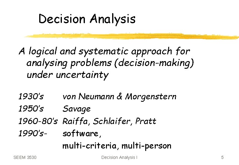
Decision Analysis A logical and systematic approach for analysing problems (decision-making) under uncertainty 1930’s 1950’s 1960 -80’s 1990’s. SEEM 3530 von Neumann & Morgenstern Savage Raiffa, Schlaifer, Pratt software, multi-criteria, multi-person Decision Analysis I 5

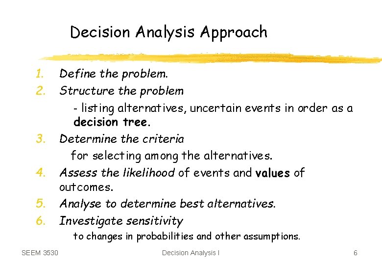
Decision Analysis Approach 1. 2. 3. 4. 5. 6. Define the problem. Structure the problem - listing alternatives, uncertain events in order as a decision tree. Determine the criteria for selecting among the alternatives. Assess the likelihood of events and values of outcomes. Analyse to determine best alternatives. Investigate sensitivity to changes in probabilities and other assumptions. SEEM 3530 Decision Analysis I 6

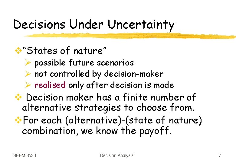
Decisions Under Uncertainty v“States of nature” Ø possible future scenarios Ø not controlled by decision-maker Ø realised only after decision is made v Decision maker has a finite number of alternative strategies to choose from. v. For each (alternative)-(state of nature) combination, we know the payoff. SEEM 3530 Decision Analysis I 7

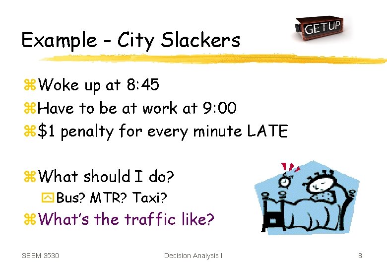
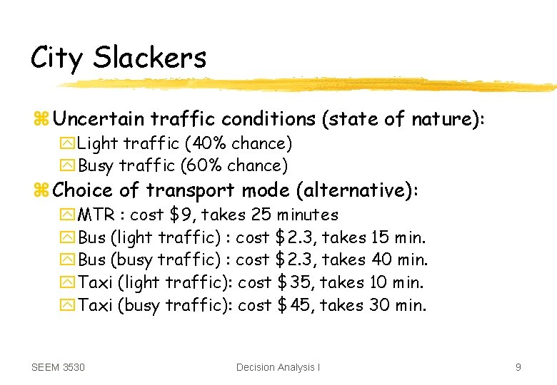
Example - City Slackers z. Woke up at 8: 45 z. Have to be at work at 9: 00 z$1 penalty for every minute LATE z. What should I do? y. Bus? MTR? Taxi? z. What’s the traffic like? SEEM 3530 Decision Analysis I 8

City Slackers z Uncertain traffic conditions (state of nature): y. Light traffic (40% chance) y. Busy traffic (60% chance) z Choice of transport mode (alternative): y. MTR : cost $9, takes 25 minutes y. Bus (light traffic) : cost $2. 3, takes 15 min. y. Bus (busy traffic) : cost $2. 3, takes 40 min. y. Taxi (light traffic): cost $35, takes 10 min. y. Taxi (busy traffic): cost $45, takes 30 min. SEEM 3530 Decision Analysis I 9

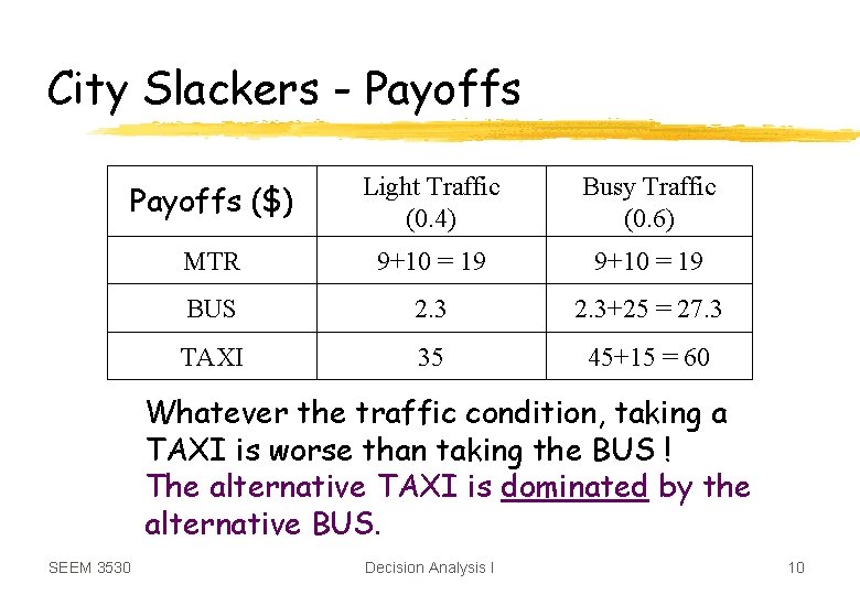
City Slackers - Payoffs ($) Light Traffic (0. 4) Busy Traffic (0. 6) MTR 9+10 = 19 BUS 2. 3+25 = 27. 3 TAXI 35 45+15 = 60 Whatever the traffic condition, taking a TAXI is worse than taking the BUS ! The alternative TAXI is dominated by the alternative BUS. SEEM 3530 Decision Analysis I 10

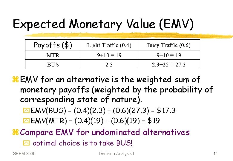
Expected Monetary Value (EMV) Payoffs ($) Light Traffic (0. 4) Busy Traffic (0. 6) MTR 9+10 = 19 BUS 2. 3+25 = 27. 3 z EMV for an alternative is the weighted sum of monetary payoffs (weighted by the probability of corresponding state of nature). y. EMV(BUS) = (0. 4)(2. 3) + (0. 6)(27. 3) = $17. 3 y. EMV(MTR) = (0. 4)(19) + (0. 6)(19) = $19 z Compare EMV for undominated alternatives y optimal choice is to take BUS! SEEM 3530 Decision Analysis I 11

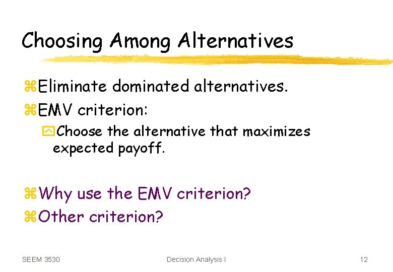
Choosing Among Alternatives z. Eliminate dominated alternatives. z. EMV criterion: y. Choose the alternative that maximizes expected payoff. z. Why use the EMV criterion? z. Other criterion? SEEM 3530 Decision Analysis I 12

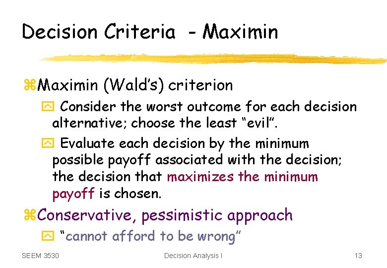
Decision Criteria - Maximin z. Maximin (Wald’s) criterion y Consider the worst outcome for each decision alternative; choose the least “evil”. y Evaluate each decision by the minimum possible payoff associated with the decision; the decision that maximizes the minimum payoff is chosen. z. Conservative, pessimistic approach y “cannot afford to be wrong” SEEM 3530 Decision Analysis I 13

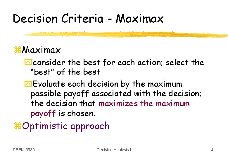
Decision Criteria - Maximax z. Maximax yconsider the best for each action; select the “best” of the best y. Evaluate each decision by the maximum possible payoff associated with the decision; the decision that maximizes the maximum payoff is chosen. z. Optimistic approach SEEM 3530 Decision Analysis I 14

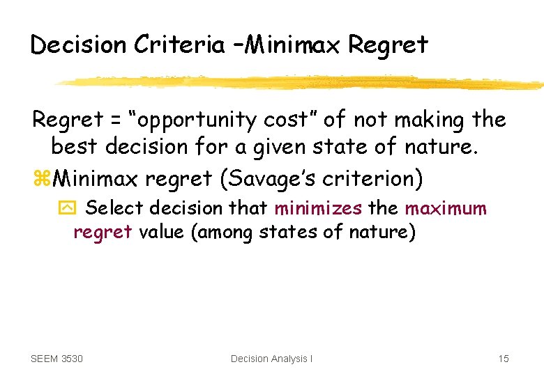
Decision Criteria –Minimax Regret = “opportunity cost” of not making the best decision for a given state of nature. z. Minimax regret (Savage’s criterion) y Select decision that minimizes the maximum regret value (among states of nature) SEEM 3530 Decision Analysis I 15

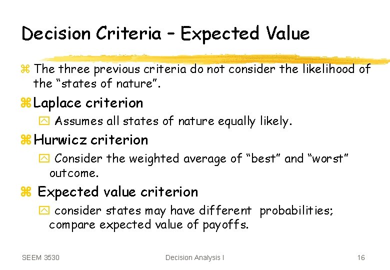
Decision Criteria – Expected Value z The three previous criteria do not consider the likelihood of the “states of nature”. z Laplace criterion y Assumes all states of nature equally likely. z Hurwicz criterion y Consider the weighted average of “best” and “worst” outcome. z Expected value criterion y consider states may have different probabilities; compare expected value of payoffs. SEEM 3530 Decision Analysis I 16

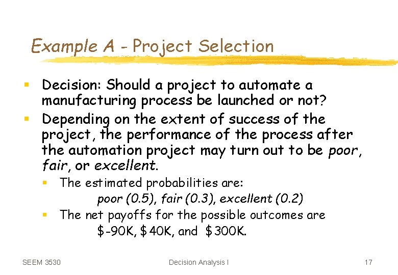
Example A - Project Selection § Decision: Should a project to automate a manufacturing process be launched or not? § Depending on the extent of success of the project, the performance of the process after the automation project may turn out to be poor, fair, or excellent. § The estimated probabilities are: poor (0. 5), fair (0. 3), excellent (0. 2) § The net payoffs for the possible outcomes are $-90 K, $40 K, and $300 K. SEEM 3530 Decision Analysis I 17

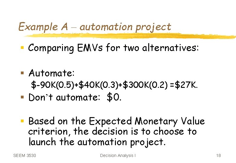
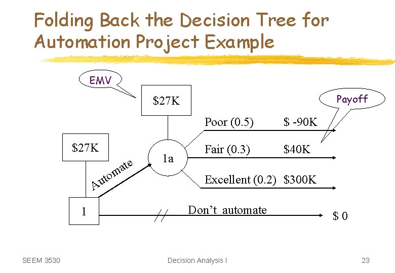
Example A – automation project § Comparing EMVs for two alternatives: § Automate: $-90 K(0. 5)+$40 K(0. 3)+$300 K(0. 2) =$27 K. § Don’t automate: $0. § Based on the Expected Monetary Value criterion, the decision is to choose to launch the automation project. SEEM 3530 Decision Analysis I 18

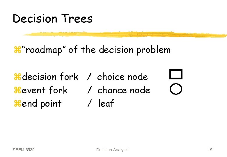
Decision Trees z“roadmap” of the decision problem zdecision fork / choice node zevent fork / chance node zend point / leaf SEEM 3530 Decision Analysis I 19

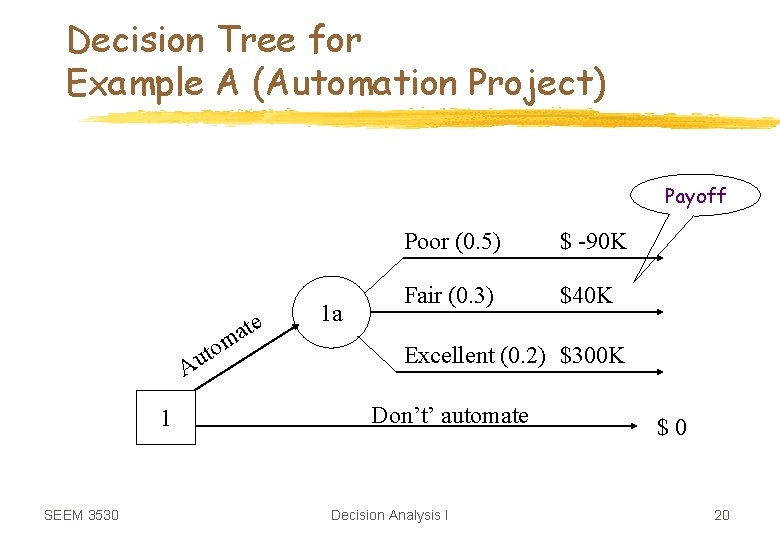
Decision Tree for Example A (Automation Project) Payoff m o t u A 1 SEEM 3530 ate 1 a Poor (0. 5) $ -90 K Fair (0. 3) $40 K Excellent (0. 2) $300 K Don’t’ automate Decision Analysis I $0 20

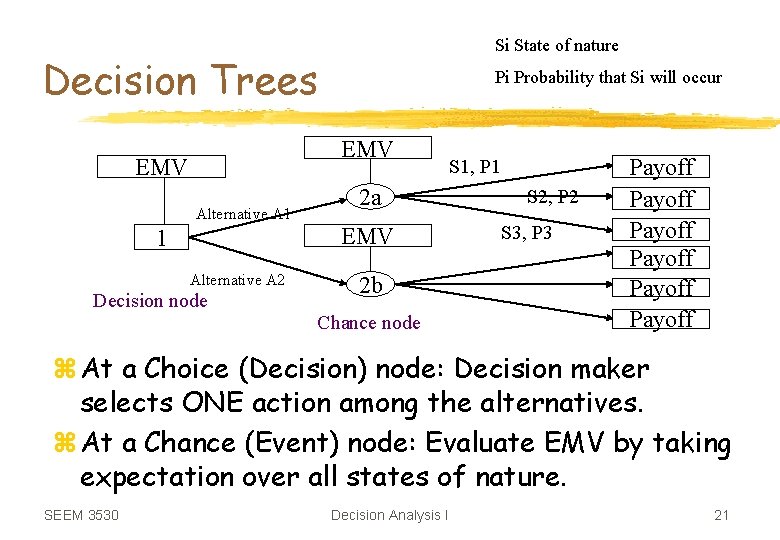
Si State of nature Decision Trees Pi Probability that Si will occur EMV Alternative A 1 2 a EMV 1 Alternative A 2 Decision node 2 b Chance node S 1, P 1 S 2, P 2 S 3, P 3 Payoff Payoff z At a Choice (Decision) node: Decision maker selects ONE action among the alternatives. z At a Chance (Event) node: Evaluate EMV by taking expectation over all states of nature. SEEM 3530 Decision Analysis I 21

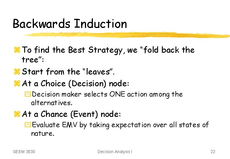
Backwards Induction z To find the Best Strategy, we “fold back the tree”: z Start from the “leaves”. z At a Choice (Decision) node: y. Decision maker selects ONE action among the alternatives. z At a Chance (Event) node: y. Evaluate EMV by taking expectation over all states of nature. SEEM 3530 Decision Analysis I 22

Folding Back the Decision Tree for Automation Project Example EMV Payoff $27 K m o t u A 1 SEEM 3530 ate 1 a Poor (0. 5) $ -90 K Fair (0. 3) $40 K Excellent (0. 2) $300 K Don’t automate Decision Analysis I $0 23

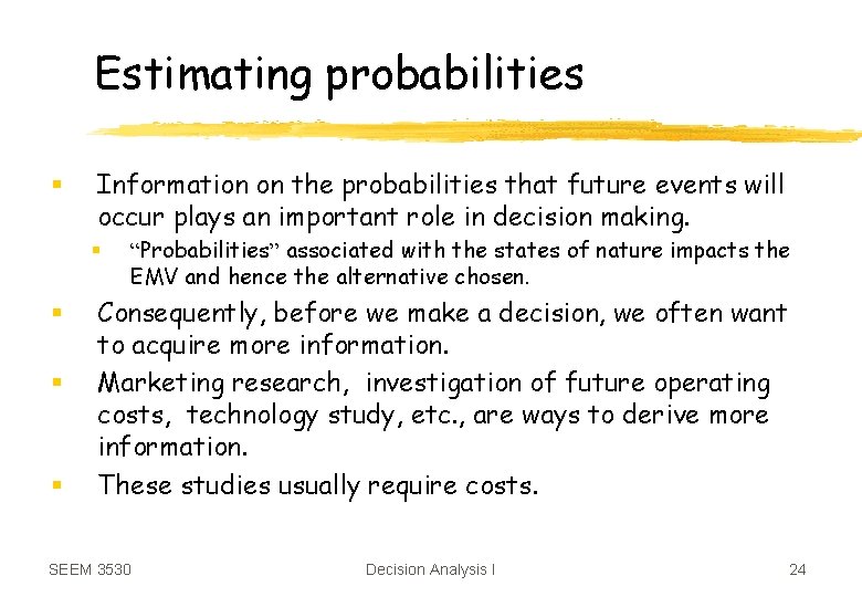
Estimating probabilities § Information on the probabilities that future events will occur plays an important role in decision making. § § “Probabilities” associated with the states of nature impacts the EMV and hence the alternative chosen. Consequently, before we make a decision, we often want to acquire more information. Marketing research, investigation of future operating costs, technology study, etc. , are ways to derive more information. These studies usually require costs. SEEM 3530 Decision Analysis I 24

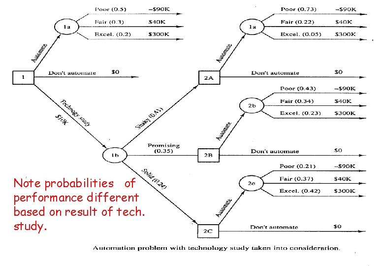
Example B (The automation project with technology study) § Suppose now it is possible to conduct a technology study at the cost of $10 K. The study will disclose that the enabling technology for the automation project is either “shaky”, “promising”, or “solid”. § The decision tree with alternative of doing a technology study and associated probabilities follows. SEEM 3530 Decision Analysis I 25

Note probabilities of performance different based on result of tech. study. SEEM 3530 Decision Analysis I 26

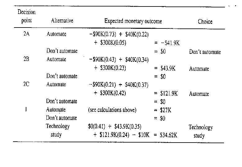
The solution to the problem: SEEM 3530 Decision Analysis I 27

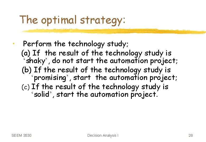
The optimal strategy: • Perform the technology study; (a) If the result of the technology study is ‘shaky’, do not start the automation project; (b) If the result of the technology study is ‘promising’, start the automation project; (c) If the result of the technology study is ‘solid’, start the automation project. SEEM 3530 Decision Analysis I 28

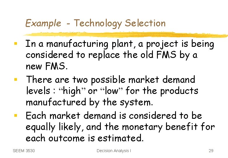
Example - Technology Selection § In a manufacturing plant, a project is being considered to replace the old FMS by a new FMS. § There are two possible market demand levels : “high” or “low” for the products manufactured by the system. § Each market demand is considered to be equally likely, and the monetary benefit for each outcome is estimated. SEEM 3530 Decision Analysis I 29

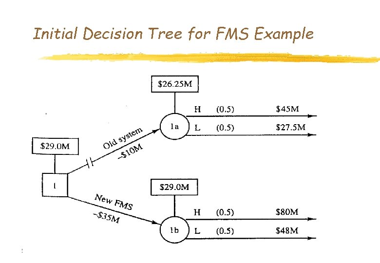
Initial Decision Tree for FMS Example SEEM 3530 Decision Analysis I 30

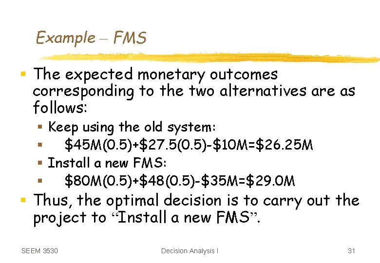
Example – FMS § The expected monetary outcomes corresponding to the two alternatives are as follows: § Keep using the old system: § $45 M(0. 5)+$27. 5(0. 5)-$10 M=$26. 25 M § Install a new FMS: § $80 M(0. 5)+$48(0. 5)-$35 M=$29. 0 M § Thus, the optimal decision is to carry out the project to “Install a new FMS”. SEEM 3530 Decision Analysis I 31

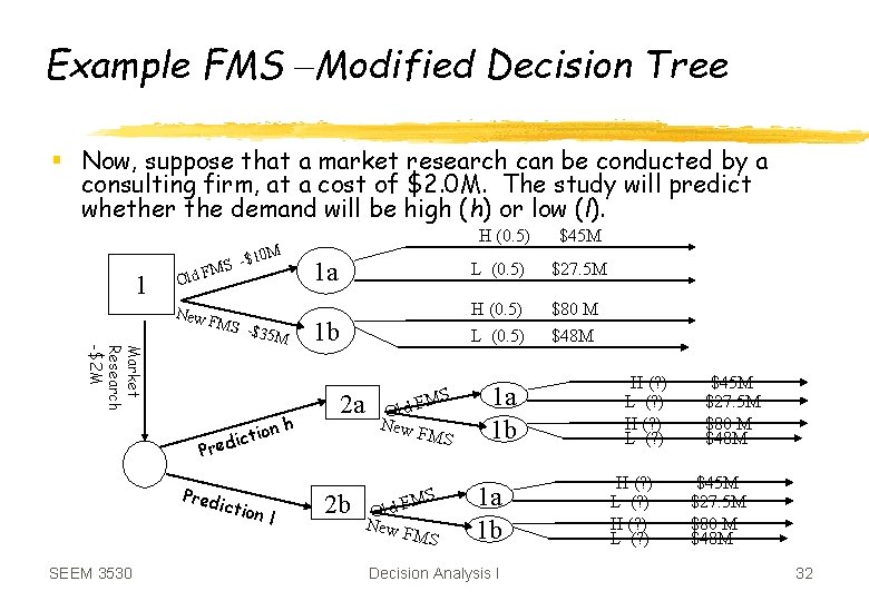
Example FMS –Modified Decision Tree § Now, suppose that a market research can be conducted by a consulting firm, at a cost of $2. 0 M. The study will predict whether the demand will be high (h) or low (l). 1 M -$10 S FM Old New F Market Research -$2 M MS $35 M nh H (0. 5) 1 a L (0. 5) $27. 5 M 1 b H (0. 5) L (0. 5) $80 M $48 M 2 a ctio i d e r P Pred ictio SEEM 3530 nl $45 M 2 b FMS d l O New F MS 1 a 1 b Decision Analysis I H (? ) L (? ) $45 M $27. 5 M $80 M $48 M 32

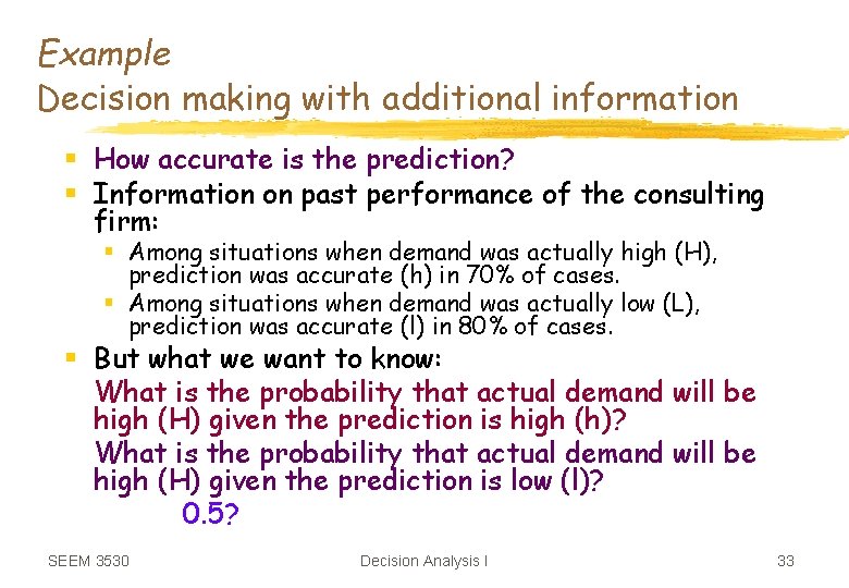
Example Decision making with additional information § How accurate is the prediction? § Information on past performance of the consulting firm: § Among situations when demand was actually high (H), prediction was accurate (h) in 70% of cases. § Among situations when demand was actually low (L), prediction was accurate (l) in 80% of cases. § But what we want to know: What is the probability that actual demand will be high (H) given the prediction is high (h)? What is the probability that actual demand will be high (H) given the prediction is low (l)? 0. 5? SEEM 3530 Decision Analysis I 33

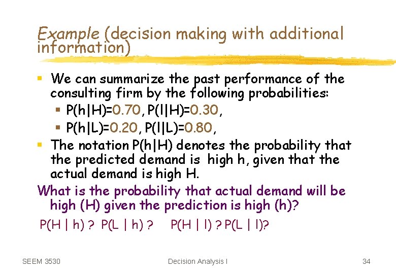
Example (decision making with additional information) § We can summarize the past performance of the consulting firm by the following probabilities: § P(h|H)=0. 70, P(l|H)=0. 30, § P(h|L)=0. 20, P(l|L)=0. 80, § The notation P(h|H) denotes the probability that the predicted demand is high h, given that the actual demand is high H. What is the probability that actual demand will be high (H) given the prediction is high (h)? P(H | h) ? P(L | h) ? SEEM 3530 P(H | l) ? P(L | l)? Decision Analysis I 34

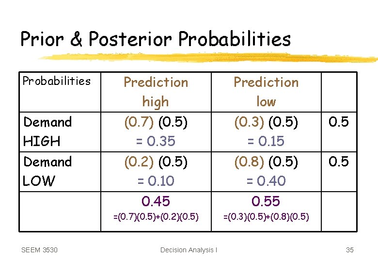
Prior & Posterior Probabilities Demand HIGH Demand LOW SEEM 3530 Prediction high (0. 7) (0. 5) = 0. 35 (0. 2) (0. 5) = 0. 10 0. 45 Prediction low (0. 3) (0. 5) = 0. 15 (0. 8) (0. 5) = 0. 40 0. 55 =(0. 7)(0. 5)+(0. 2)(0. 5) =(0. 3)(0. 5)+(0. 8)(0. 5) Decision Analysis I 0. 5 35

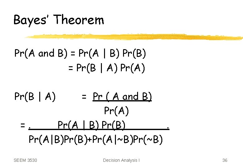
Bayes’ Theorem Pr(A and B) = Pr(A | B) Pr(B) = Pr(B | A) = Pr ( A and B) Pr(A) =. Pr(A | B) Pr(B). Pr(A|B)Pr(B)+Pr(A|~B)Pr(~B) SEEM 3530 Decision Analysis I 36

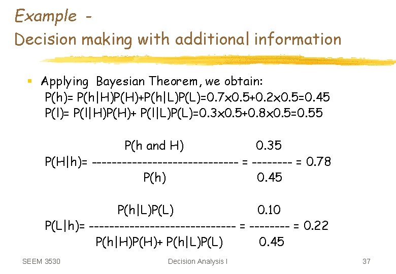
Example Decision making with additional information § Applying Bayesian Theorem, we obtain: P(h)= P(h|H)P(H)+P(h|L)P(L)=0. 7 x 0. 5+0. 2 x 0. 5=0. 45 P(l)= P(l|H)P(H)+ P(l|L)P(L)=0. 3 x 0. 5+0. 8 x 0. 5=0. 55 P(h and H) 0. 35 P(H|h)= --------------- = 0. 78 P(h) 0. 45 P(h|L)P(L) 0. 10 P(L|h)= --------------- = 0. 22 P(h|H)P(H)+ P(h|L)P(L) 0. 45 SEEM 3530 Decision Analysis I 37

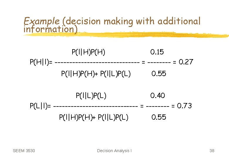
Example (decision making with additional information) P(l|H)P(H) 0. 15 P(H|l)= --------------- = 0. 27 P(l|H)P(H)+ P(l|L)P(L) 0. 55 P(l|L)P(L) 0. 40 P(L|l)= --------------- = 0. 73 P(l|H)P(H)+ P(l|L)P(L) SEEM 3530 Decision Analysis I 0. 55 38

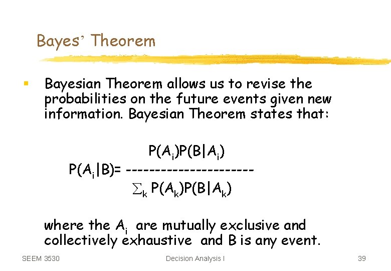
Bayes’ Theorem § Bayesian Theorem allows us to revise the probabilities on the future events given new information. Bayesian Theorem states that: P(Ai)P(B|Ai) P(Ai|B)= ----------- k P(Ak)P(B|Ak) where the Ai are mutually exclusive and collectively exhaustive and B is any event. SEEM 3530 Decision Analysis I 39

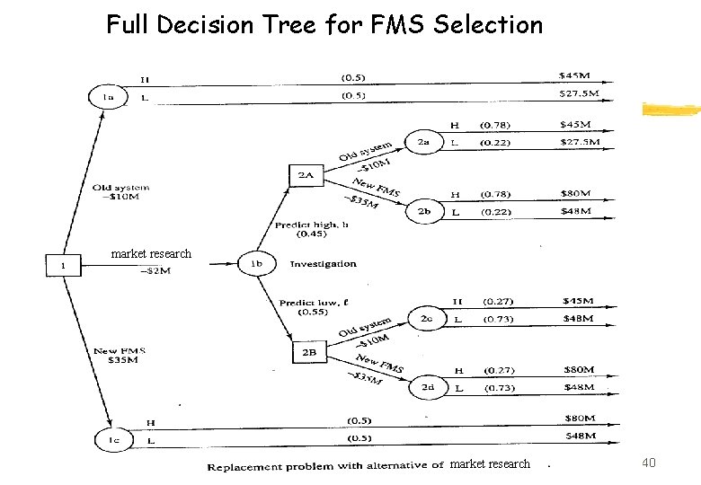
Full Decision Tree for FMS Selection market research SEEM 3530 Decision Analysis I market research 40

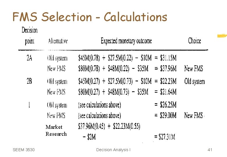
FMS Selection - Calculations Market Research SEEM 3530 Decision Analysis I 41

FMS - The optimal decision § The optimal decision according to the decision tree analysis is to go ahead with the project to install a new FMS (without employing the consulting firm to conduct the market research), which gives an expected income $29. 0 M. SEEM 3530 Decision Analysis I 42

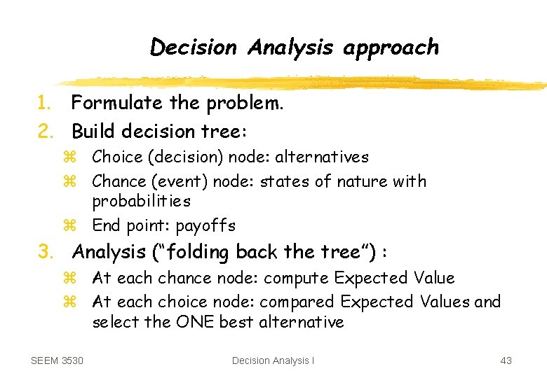
Decision Analysis approach 1. Formulate the problem. 2. Build decision tree: z Choice (decision) node: alternatives z Chance (event) node: states of nature with probabilities z End point: payoffs 3. Analysis (“folding back the tree”) : z At each chance node: compute Expected Value z At each choice node: compared Expected Values and select the ONE best alternative SEEM 3530 Decision Analysis I 43

Summary z Decision Trees: y. Choice/decision node y. Chance/event node y. Leaf/end point y. Payoff/outcome values y. Probabilities for outcomes/states of nature y. Criterion e. g. EMV y. Folding Back the Tree y. Strategy z Bayes’ Theorem yconditional probabilities SEEM 3530 Decision Analysis I 44