Chapter 14 Decision Analysis Decision Making Many decision

Chapter 14 Decision Analysis

Decision Making • Many decision making occur under condition of uncertainty • Decision situations – Probability cannot be assigned to future occurrence

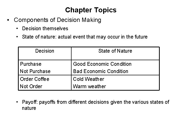
Chapter Topics • Components of Decision Making • Decision themselves • State of nature: actual event that may occur in the future Decision State of Nature Purchase Not Purchase Good Economic Condition Bad Economic Condition Order Coffee Not Order Cold Weather Warm weather • Payoff: payoffs from different decisions given the various states of nature

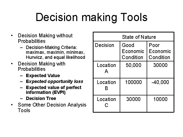
Decision making Tools • Decision Making without Probabilities – Decision-Making Criteria: maximax, maximin, minimax, Hurwicz, and equal likelihood • Decision Making with Probabilities – Expected Value – Expected opportunity loss – Expected value of perfect information (EVPI) – Decision Tree • Some Other Decision Analysis Tools State of Nature Decision Good Poor Economic Condition Location A 50, 000 30000 Location B 100000 -40, 000 Location C 30000 10000

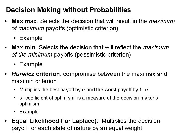
Decision Making without Probabilities • Maximax: Selects the decision that will result in the maximum of maximum payoffs (optimistic criterion) • Example • Maximin: Selects the decision that will reflect the maximum of the minimum payoffs (pessimistic criterion) • Example • Hurwicz criterion: compromise between the maximax and maximin criterion • Multiplies the best payoff by and the worst payoff by 1 - • , coefficient of optimism, is a measure of the decision maker’s optimism • Example • Equal Likelihood ( or Laplace): Multiplies the decision payoff for each state of nature by an equal weight

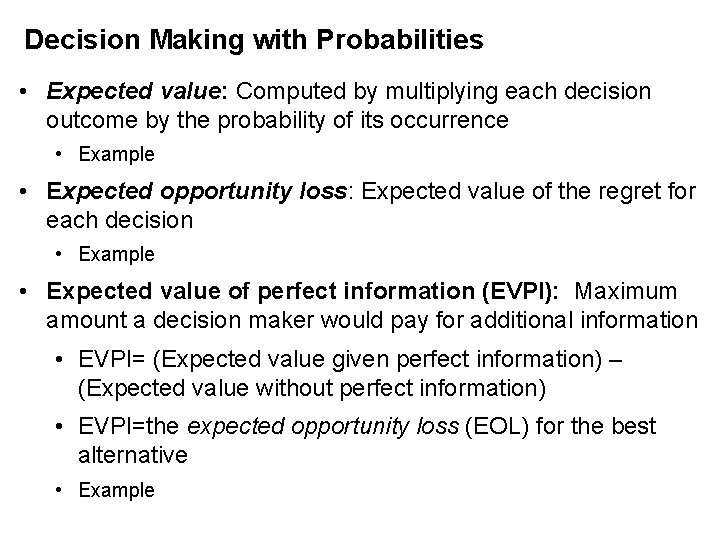
Decision Making with Probabilities • Expected value: Computed by multiplying each decision outcome by the probability of its occurrence • Example • Expected opportunity loss: Expected value of the regret for each decision • Example • Expected value of perfect information (EVPI): Maximum amount a decision maker would pay for additional information • EVPI= (Expected value given perfect information) – (Expected value without perfect information) • EVPI=the expected opportunity loss (EOL) for the best alternative • Example

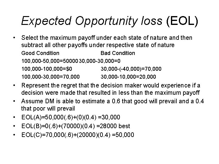
Expected Opportunity loss (EOL) • Select the maximum payoff under each state of nature and then subtract all other payoffs under respective state of nature Good Condition Bad Condition 100, 000 -50, 000=50000 30, 000 -30, 000=0 100, 000 -100, 000=$0 30, 000 -(-40, 000)=70, 000 100, 000 -30, 000=70, 000 30, 000 -10, 000=20, 000 • Represent the regret that the decision maker would experience if a decision were made that resulted in less than the maximum payoff • Assume DM is able to estimate a 0. 6 that good will prevail and a 0. 4 that poor will prevail • EOL(A)=50, 000(. 6)+(0)(0. 4) =30, 000 • EOL(B)=0(. 6)+(70000)(0. 4) =28000 best • EOL(C)=70, 000(. 6)+(20000)(0. 4) =50, 000

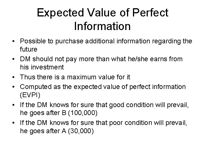
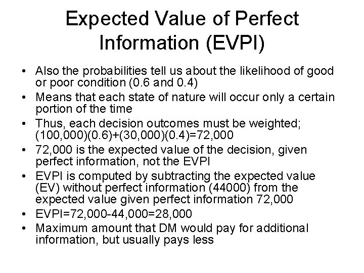
Expected Value of Perfect Information • Possible to purchase additional information regarding the future • DM should not pay more than what he/she earns from his investment • Thus there is a maximum value for it • Computed as the expected value of perfect information (EVPI) • If the DM knows for sure that good condition will prevail, he goes after B (100, 000) • If the DM knows for sure that poor condition will prevail, he goes after A (30, 000)

Expected Value of Perfect Information (EVPI) • Also the probabilities tell us about the likelihood of good or poor condition (0. 6 and 0. 4) • Means that each state of nature will occur only a certain portion of the time • Thus, each decision outcomes must be weighted; (100, 000)(0. 6)+(30, 000)(0. 4)=72, 000 • 72, 000 is the expected value of the decision, given perfect information, not the EVPI • EVPI is computed by subtracting the expected value (EV) without perfect information (44000) from the expected value given perfect information 72, 000 • EVPI=72, 000 -44, 000=28, 000 • Maximum amount that DM would pay for additional information, but usually pays less

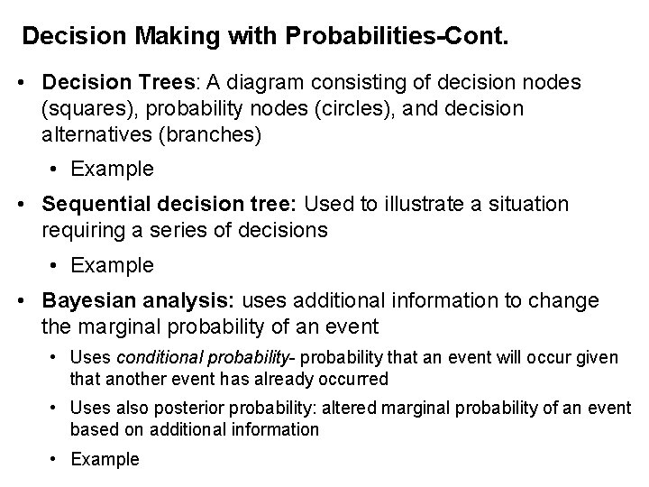
Decision Making with Probabilities-Cont. • Decision Trees: A diagram consisting of decision nodes (squares), probability nodes (circles), and decision alternatives (branches) • Example • Sequential decision tree: Used to illustrate a situation requiring a series of decisions • Example • Bayesian analysis: uses additional information to change the marginal probability of an event • Uses conditional probability- probability that an event will occur given that another event has already occurred • Uses also posterior probability: altered marginal probability of an event based on additional information • Example

Decision Analysis Example a. Determine the best decision using the 5 criteria b. Determine best decision with probabilities assuming. 70 probability of good conditions, . 30 of poor conditions. Use expected value and expected opportunity loss criteria. c. Compute expected value of perfect information. d. Develop a decision tree with expected value at the nodes e. Given following, P(P g) =. 70, P(N g) =. 30, P(P p) = 20, P(N p) =. 80, determine posteria probabilities using Bayes’ rule f. Perform a decision tree analysis using the posterior probability obtained in part e