CSC 381481 Quarter Fall 0304 Daniela Stan Raicu

CSC 381/481 Quarter: Fall 03/04 Daniela Stan Raicu Email: draicu@cs. depaul. edu Homepage: http: //facweb. cs. depaul. edu/dstan School of CTI, De. Paul University 3/10/2021 Daniela Stan - CSC 381/481 1

Outline Ø Chapter 2: Digital Image Fundamentals Ø Section 2. 4: Image sampling and quantization Ø Ø Ø Basic concepts Representing digital images Spatial and gray-level resolution Ø Section 2. 5: Some basic relationships between pixels Ø Ø Neighbors of a pixel Adjacency, connectivity, regions, and boundaries Distance measures Image operations on a pixel basis Ø Algebra review Ø Matlab tutorial 3/10/2021 Daniela Stan - CSC 381/481 2

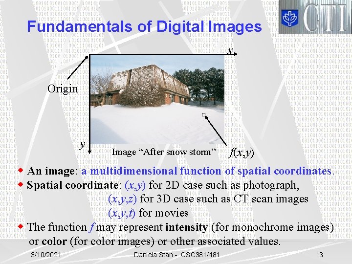
Fundamentals of Digital Images x Origin y Image “After snow storm” f(x, y) w An image: a multidimensional function of spatial coordinates. w Spatial coordinate: (x, y) for 2 D case such as photograph, (x, y, z) for 3 D case such as CT scan images (x, y, t) for movies w The function f may represent intensity (for monochrome images) or color (for color images) or other associated values. 3/10/2021 Daniela Stan - CSC 381/481 3

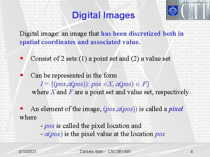
Digital Images Digital image: an image that has been discretized both in spatial coordinates and associated value. w Consist of 2 sets: (1) a point set and (2) a value set w Can be represented in the form I = {(pos, a(pos)): pos ÎX, a(pos) Î F} where X and F are a point set and value set, respectively. w An element of the image, (pos, a(pos)) is called a pixel where - pos is called the pixel location and - a(pos) is the pixel value at the location pos 3/10/2021 Daniela Stan - CSC 381/481 4

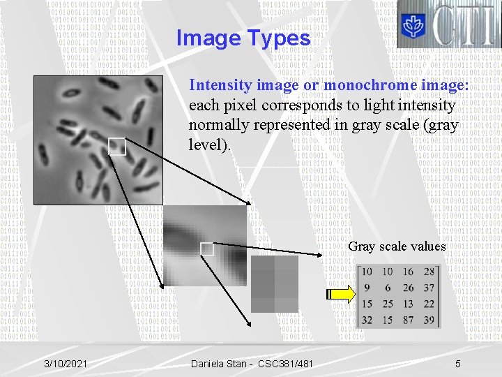
Image Types Intensity image or monochrome image: each pixel corresponds to light intensity normally represented in gray scale (gray level). Gray scale values 3/10/2021 Daniela Stan - CSC 381/481 5

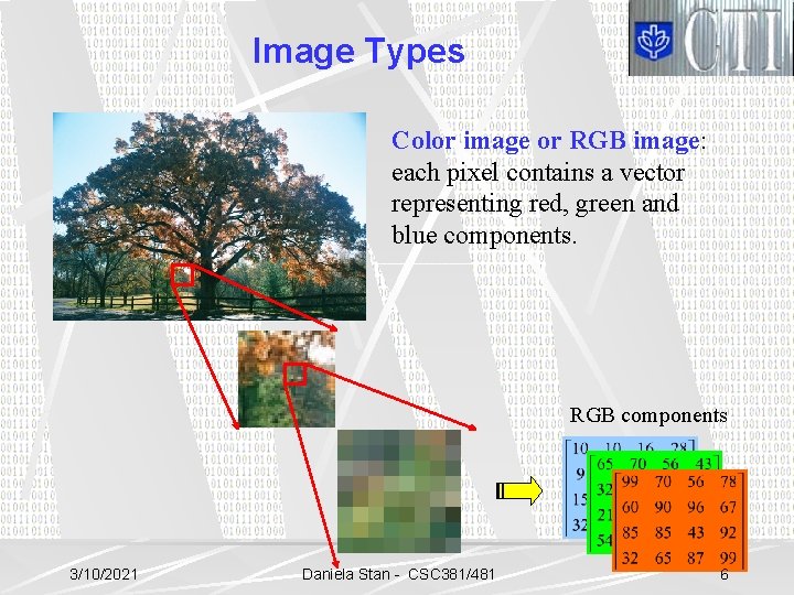
Image Types Color image or RGB image: each pixel contains a vector representing red, green and blue components. RGB components 3/10/2021 Daniela Stan - CSC 381/481 6

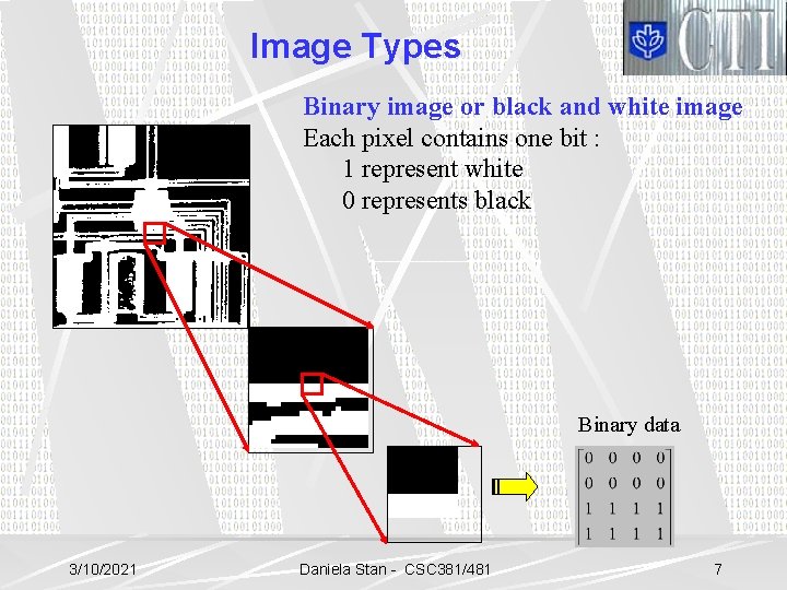
Image Types Binary image or black and white image Each pixel contains one bit : 1 represent white 0 represents black Binary data 3/10/2021 Daniela Stan - CSC 381/481 7

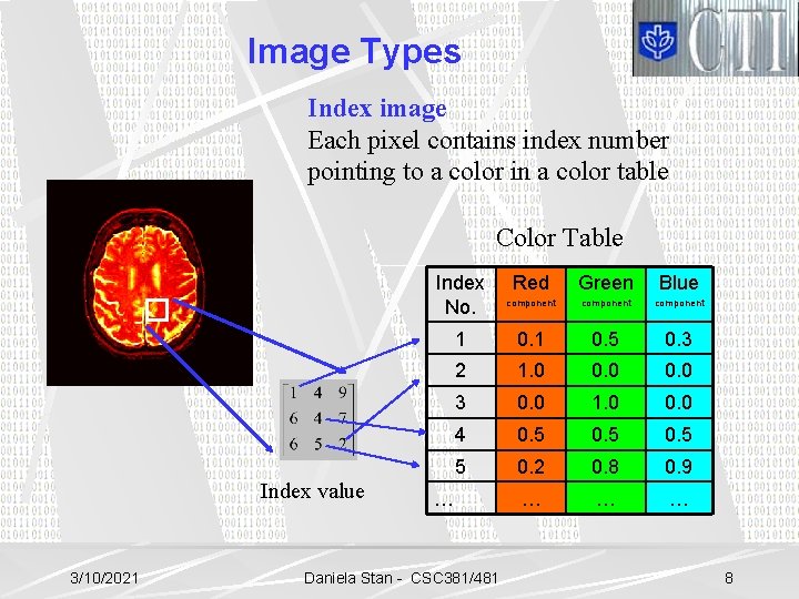
Image Types Index image Each pixel contains index number pointing to a color in a color table Color Table Index No. Index value 3/10/2021 Red Green Blue component 1 0. 5 0. 3 2 1. 0 0. 0 3 0. 0 1. 0 0. 0 4 0. 5 5 0. 2 0. 8 0. 9 … … Daniela Stan - CSC 381/481 8

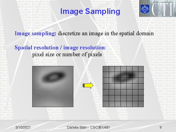
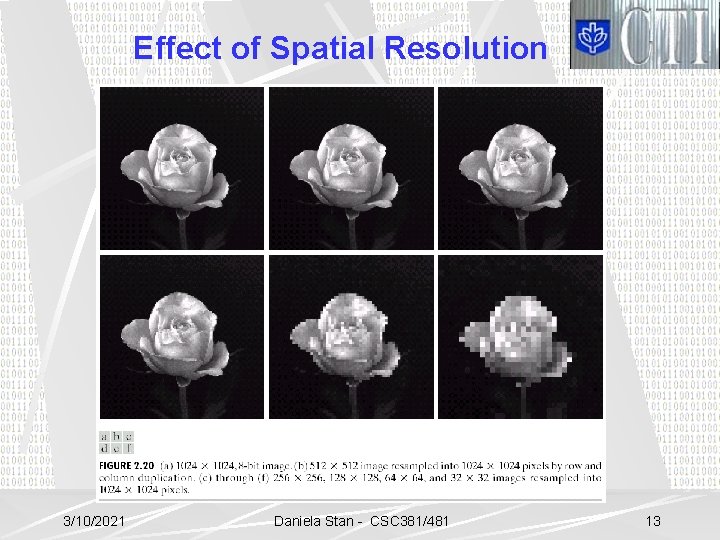
Image Sampling Image sampling: discretize an image in the spatial domain Spatial resolution / image resolution: pixel size or number of pixels 3/10/2021 Daniela Stan - CSC 381/481 9

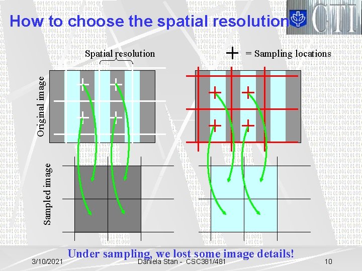
How to choose the spatial resolution = Sampling locations Sampled image Original image Spatial resolution 3/10/2021 Under sampling, we lost some image details! Daniela Stan - CSC 381/481 10

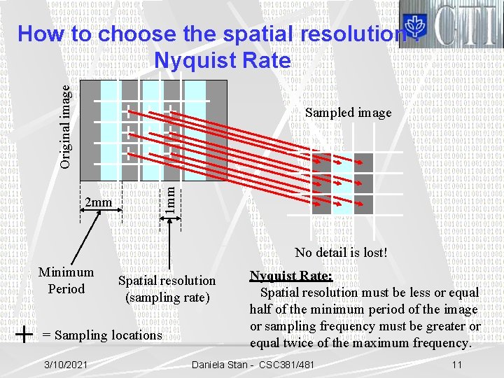
Original image How to choose the spatial resolution : Nyquist Rate 2 mm 1 mm Sampled image No detail is lost! Minimum Period Spatial resolution (sampling rate) = Sampling locations 3/10/2021 Nyquist Rate: Spatial resolution must be less or equal half of the minimum period of the image or sampling frequency must be greater or equal twice of the maximum frequency. Daniela Stan - CSC 381/481 11

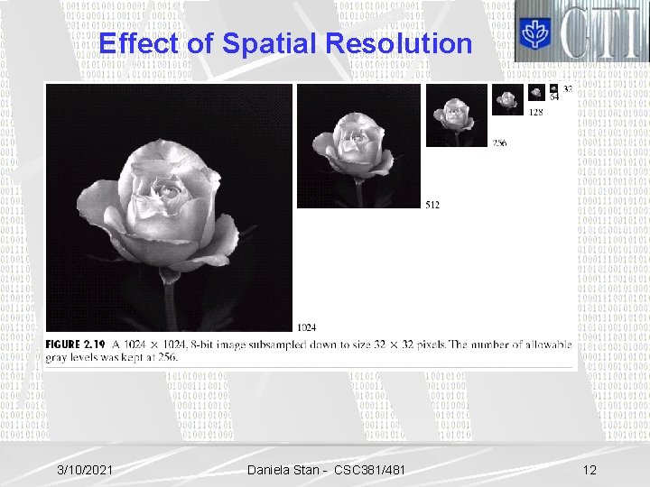
Effect of Spatial Resolution 3/10/2021 Daniela Stan - CSC 381/481 12

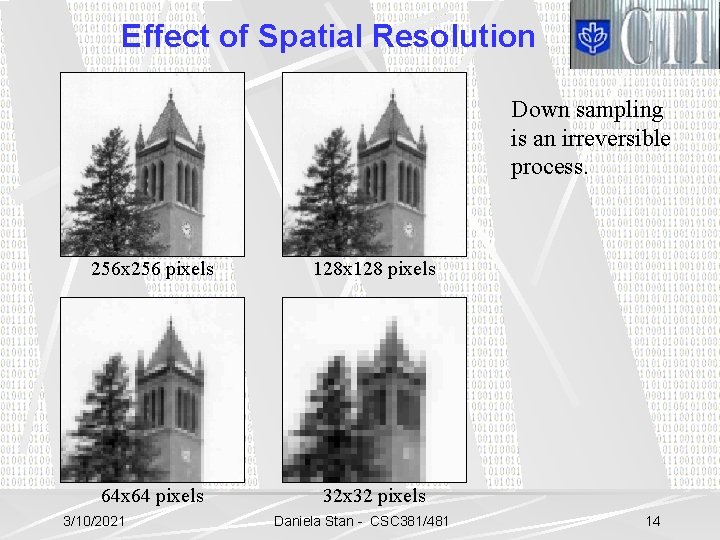
Effect of Spatial Resolution 3/10/2021 Daniela Stan - CSC 381/481 13

Effect of Spatial Resolution Down sampling is an irreversible process. 256 x 256 pixels 128 x 128 pixels 64 x 64 pixels 32 x 32 pixels 3/10/2021 Daniela Stan - CSC 381/481 14

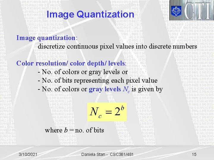
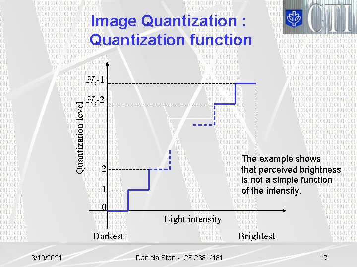
Image Quantization Image quantization: discretize continuous pixel values into discrete numbers Color resolution/ color depth/ levels: - No. of colors or gray levels or - No. of bits representing each pixel value - No. of colors or gray levels Nc is given by where b = no. of bits 3/10/2021 Daniela Stan - CSC 381/481 15

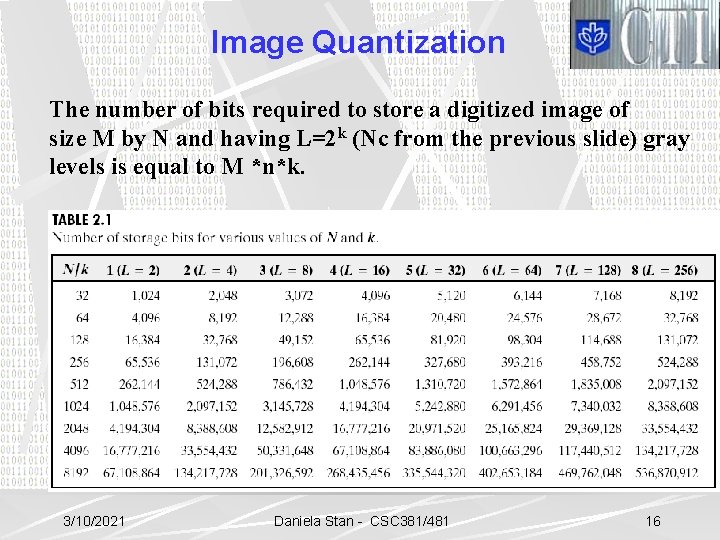
Image Quantization The number of bits required to store a digitized image of size M by N and having L=2 k (Nc from the previous slide) gray levels is equal to M *n*k. 3/10/2021 Daniela Stan - CSC 381/481 16

Image Quantization : Quantization function Quantization level Nc-1 Nc-2 The example shows that perceived brightness is not a simple function of the intensity. 2 1 0 Light intensity Darkest 3/10/2021 Brightest Daniela Stan - CSC 381/481 17

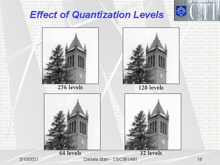
Effect of Quantization Levels 3/10/2021 256 levels 128 levels 64 levels 32 levels Daniela Stan - CSC 381/481 18

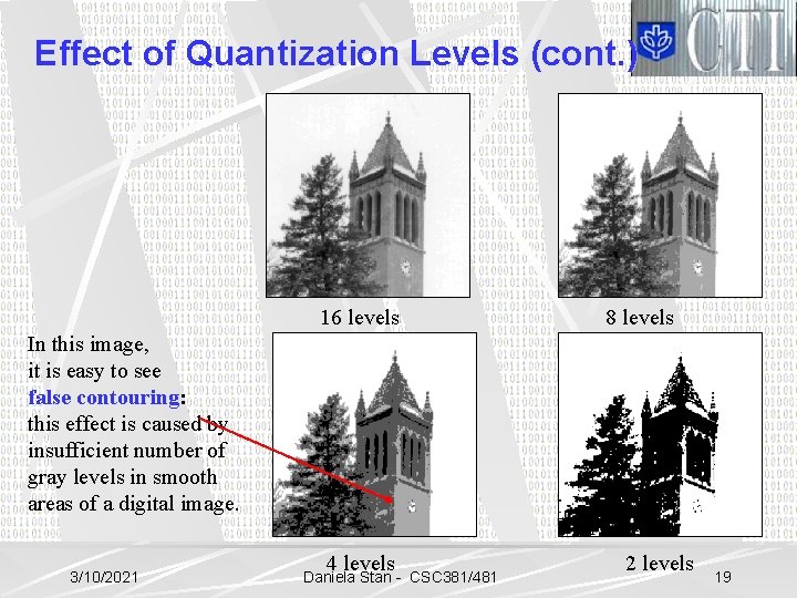
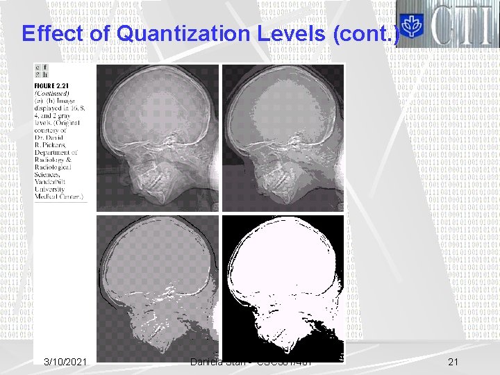
Effect of Quantization Levels (cont. ) 16 levels 8 levels In this image, it is easy to see false contouring: this effect is caused by insufficient number of gray levels in smooth areas of a digital image. 3/10/2021 4 levels Daniela Stan - CSC 381/481 2 levels 19

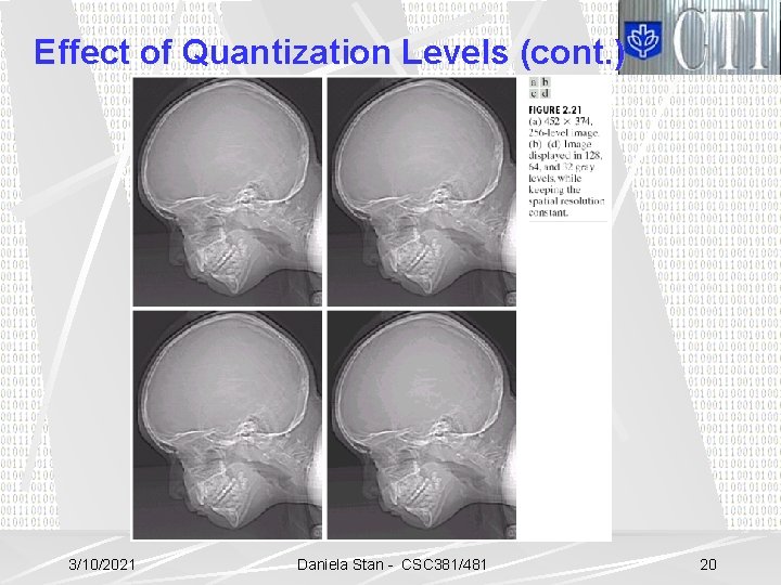
Effect of Quantization Levels (cont. ) 3/10/2021 Daniela Stan - CSC 381/481 20

Effect of Quantization Levels (cont. ) 3/10/2021 Daniela Stan - CSC 381/481 21

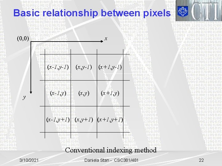
Basic relationship between pixels (0, 0) y x (x-1, y-1) (x+1, y-1) (x-1, y) (x+1, y) (x-1, y+1) (x+1, y+1) Conventional indexing method 3/10/2021 Daniela Stan - CSC 381/481 22

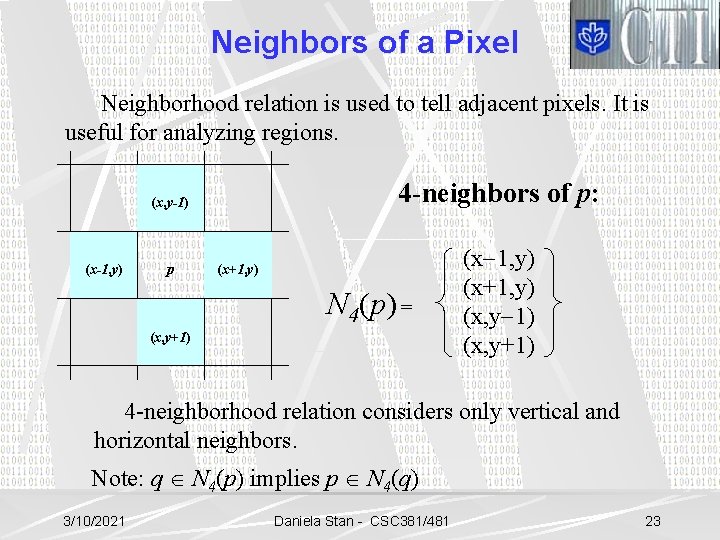
Neighbors of a Pixel Neighborhood relation is used to tell adjacent pixels. It is useful for analyzing regions. 4 -neighbors of p: (x, y-1) (x-1, y) p (x+1, y) N 4(p) = (x, y+1) (x-1, y) (x+1, y) (x, y-1) (x, y+1) 4 -neighborhood relation considers only vertical and horizontal neighbors. Note: q Î N 4(p) implies p Î N 4(q) 3/10/2021 Daniela Stan - CSC 381/481 23

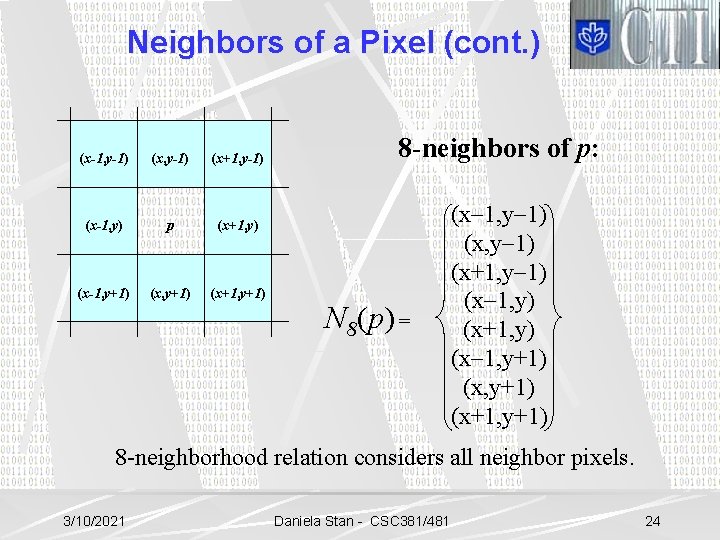
Neighbors of a Pixel (cont. ) (x-1, y-1) (x+1, y-1) (x-1, y) p (x+1, y) (x-1, y+1) (x+1, y+1) 8 -neighbors of p: N 8(p) = (x-1, y-1) (x+1, y-1) (x-1, y) (x+1, y) (x-1, y+1) (x+1, y+1) 8 -neighborhood relation considers all neighbor pixels. 3/10/2021 Daniela Stan - CSC 381/481 24

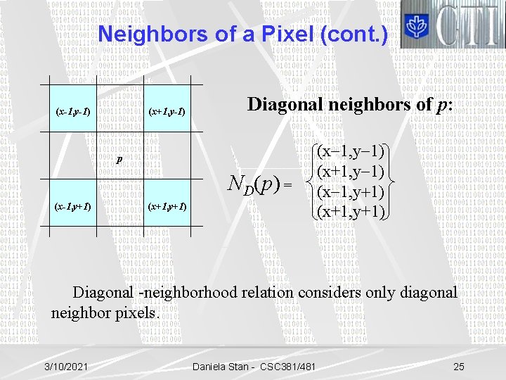
Neighbors of a Pixel (cont. ) (x-1, y-1) (x+1, y-1) Diagonal neighbors of p: p ND(p) = (x-1, y+1) (x+1, y+1) (x-1, y-1) (x+1, y-1) (x-1, y+1) (x+1, y+1) Diagonal -neighborhood relation considers only diagonal neighbor pixels. 3/10/2021 Daniela Stan - CSC 381/481 25

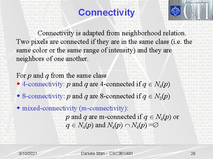
Connectivity is adapted from neighborhood relation. Two pixels are connected if they are in the same class (i. e. the same color or the same range of intensity) and they are neighbors of one another. For p and q from the same class w 4 -connectivity: p and q are 4 -connected if q Î N 4(p) w 8 -connectivity: p and q are 8 -connected if q Î N 8(p) w mixed-connectivity (m-connectivity): p and q are m-connected if q Î N 4(p) or q Î N 4(p) and N 4(p) Ç N 4(p) =Æ 3/10/2021 Daniela Stan - CSC 381/481 26

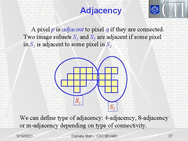
Adjacency A pixel p is adjacent to pixel q if they are connected. Two image subsets S 1 and S 2 are adjacent if some pixel in S 1 is adjacent to some pixel in S 2 S 1 S 2 We can define type of adjacency: 4 -adjacency, 8 -adjacency or m-adjacency depending on type of connectivity. 3/10/2021 Daniela Stan - CSC 381/481 27

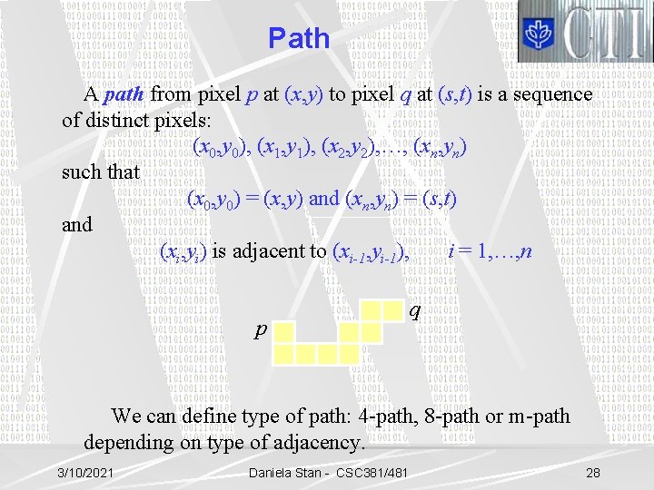
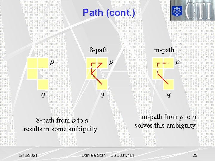
Path A path from pixel p at (x, y) to pixel q at (s, t) is a sequence of distinct pixels: (x 0, y 0), (x 1, y 1), (x 2, y 2), …, (xn, yn) such that (x 0, y 0) = (x, y) and (xn, yn) = (s, t) and (xi, yi) is adjacent to (xi-1, yi-1), i = 1, …, n p q We can define type of path: 4 -path, 8 -path or m-path depending on type of adjacency. 3/10/2021 Daniela Stan - CSC 381/481 28

Path (cont. ) 8 -path p m-path p q q 8 -path from p to q results in some ambiguity 3/10/2021 Daniela Stan - CSC 381/481 p q m-path from p to q solves this ambiguity 29

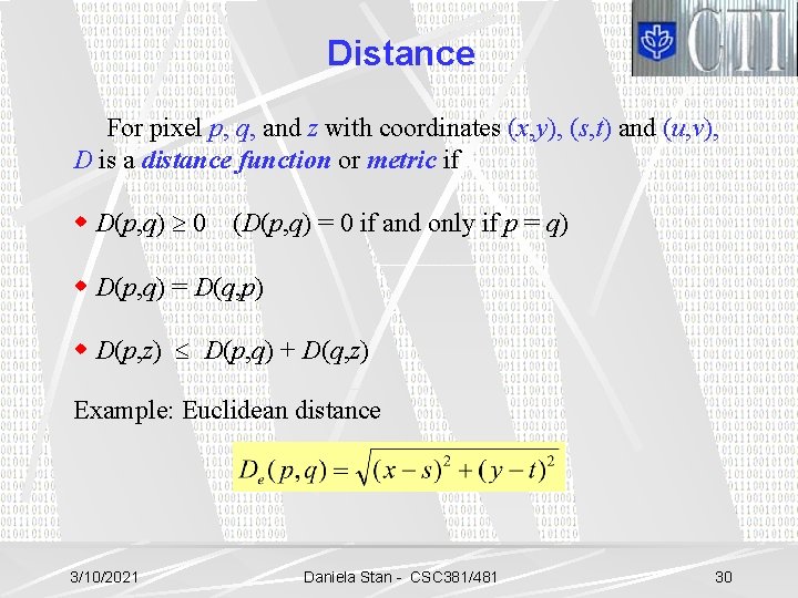
Distance For pixel p, q, and z with coordinates (x, y), (s, t) and (u, v), D is a distance function or metric if w D(p, q) ³ 0 (D(p, q) = 0 if and only if p = q) w D(p, q) = D(q, p) w D(p, z) £ D(p, q) + D(q, z) Example: Euclidean distance 3/10/2021 Daniela Stan - CSC 381/481 30

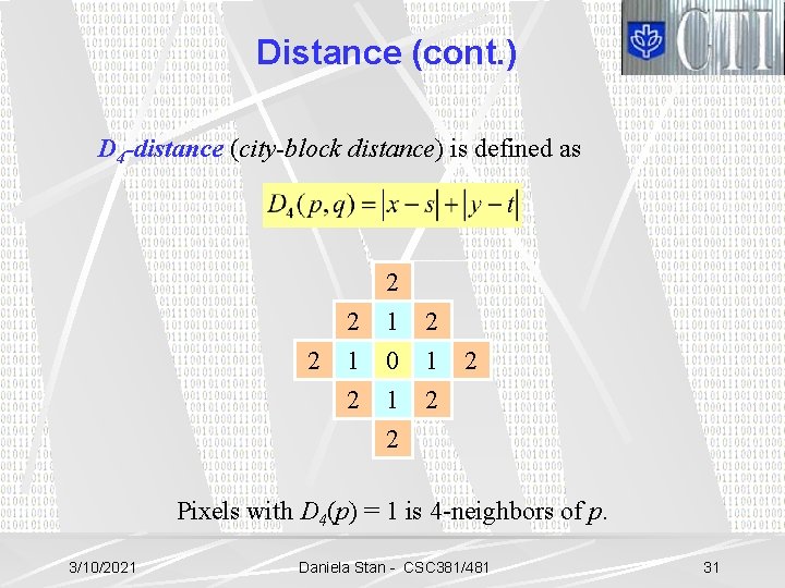
Distance (cont. ) D 4 -distance (city-block distance) is defined as 2 2 2 1 0 1 2 2 Pixels with D 4(p) = 1 is 4 -neighbors of p. 3/10/2021 Daniela Stan - CSC 381/481 31

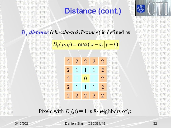
Distance (cont. ) D 8 -distance (chessboard distance) is defined as 2 2 2 2 2 1 1 1 2 1 0 1 2 1 1 1 2 2 2 Pixels with D 8(p) = 1 is 8 -neighbors of p. 3/10/2021 Daniela Stan - CSC 381/481 32

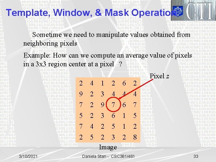
Template, Window, & Mask Operation Sometime we need to manipulate values obtained from neighboring pixels Example: How can we compute an average value of pixels in a 3 x 3 region center at a pixel z? 2 9 7 5 7 2 3/10/2021 4 2 2 2 4 5 1 2 3 4 9 7 3 6 2 5 2 3 Image 6 4 6 1 1 2 2 4 7 5 2 8 Daniela Stan - CSC 381/481 Pixel z 33

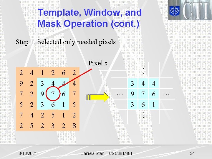
Template, Window, and Mask Operation (cont. ) Step 1. Selected only needed pixels 1 2 6 2 9 7 5 7 2 3 9 3 2 2 4 7 6 5 3 4 6 1 1 2 4 7 5 2 8 2 2 2 4 5 3/10/2021 … 3 9 3 4 7 6 4 6 1 … … 2 4 … Pixel z Daniela Stan - CSC 381/481 34

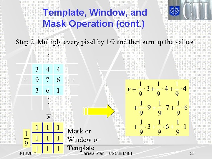
Template, Window, and Mask Operation (cont. ) … Step 2. Multiply every pixel by 1/9 and then sum up the values 4 4 9 7 6 3 6 1 … … … 3 X 1 1 1 1 1 3/10/2021 Mask or Window or Template Daniela Stan - CSC 381/481 35

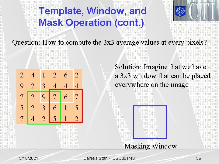
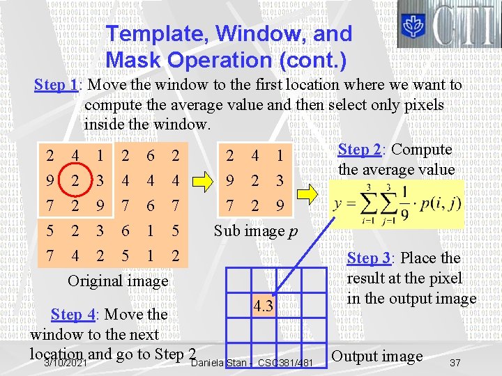
Template, Window, and Mask Operation (cont. ) Question: How to compute the 3 x 3 average values at every pixels? 2 4 1 2 6 2 9 7 5 7 3 9 3 2 4 7 6 5 4 6 1 1 4 7 5 2 2 4 Solution: Imagine that we have a 3 x 3 window that can be placed everywhere on the image Masking Window 3/10/2021 Daniela Stan - CSC 381/481 36

Template, Window, and Mask Operation (cont. ) Step 1: Move the window to the first location where we want to compute the average value and then select only pixels inside the window. Step 2: Compute 2 4 1 2 6 2 2 4 1 the average value 9 2 3 4 4 4 9 2 3 7 2 5 2 7 4 9 3 2 7 6 5 6 7 1 5 1 2 7 2 9 Sub image p Original image Step 4: Move the window to the next location and go to Step 2 Daniela Stan 3/10/2021 4. 3 CSC 381/481 Step 3: Place the result at the pixel in the output image Output image 37

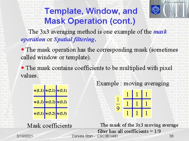
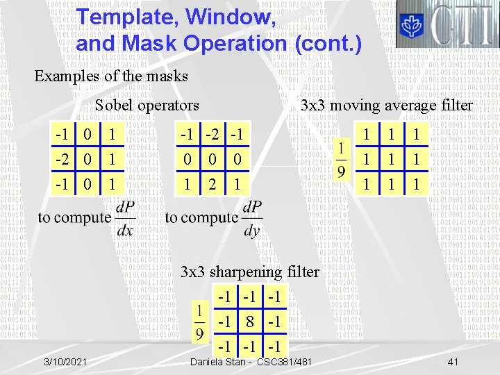
Template, Window, and Mask Operation (cont. ) The 3 x 3 averaging method is one example of the mask operation or Spatial filtering. w The mask operation has the corresponding mask (sometimes called window or template). w The mask contains coefficients to be multiplied with pixel values. Example : moving averaging w(1, 1) w(2, 1) w(3, 1) 1 1 1 w(1, 2) w(2, 2) w(3, 1) w(3, 2) w(3, 3) Mask coefficients 3/10/2021 1 1 1 The mask of the 3 x 3 moving average filter has all coefficients = 1/9 Daniela Stan - CSC 381/481 38

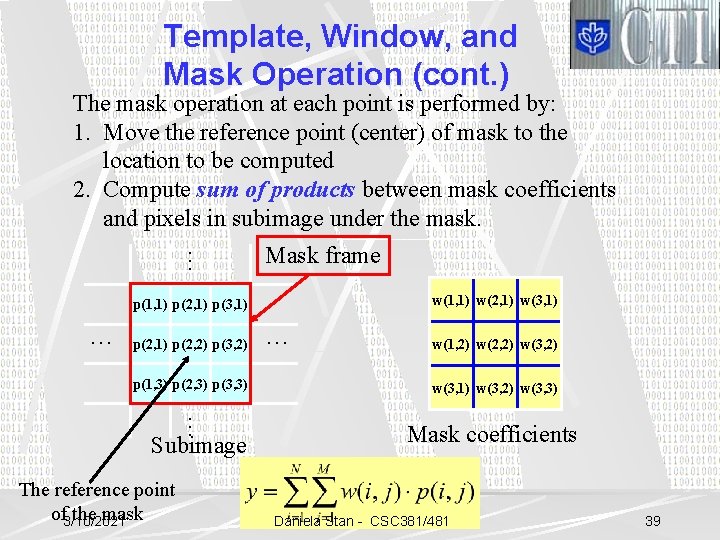
Template, Window, and Mask Operation (cont. ) … The mask operation at each point is performed by: 1. Move the reference point (center) of mask to the location to be computed 2. Compute sum of products between mask coefficients and pixels in subimage under the mask. Mask frame w(1, 1) w(2, 1) w(3, 1) p(1, 1) p(2, 1) p(3, 1) … p(2, 1) p(2, 2) p(3, 2) … p(1, 3) p(2, 3) p(3, 3) Subimage The reference point of 3/10/2021 the mask … w(1, 2) w(2, 2) w(3, 1) w(3, 2) w(3, 3) Mask coefficients Daniela Stan - CSC 381/481 39

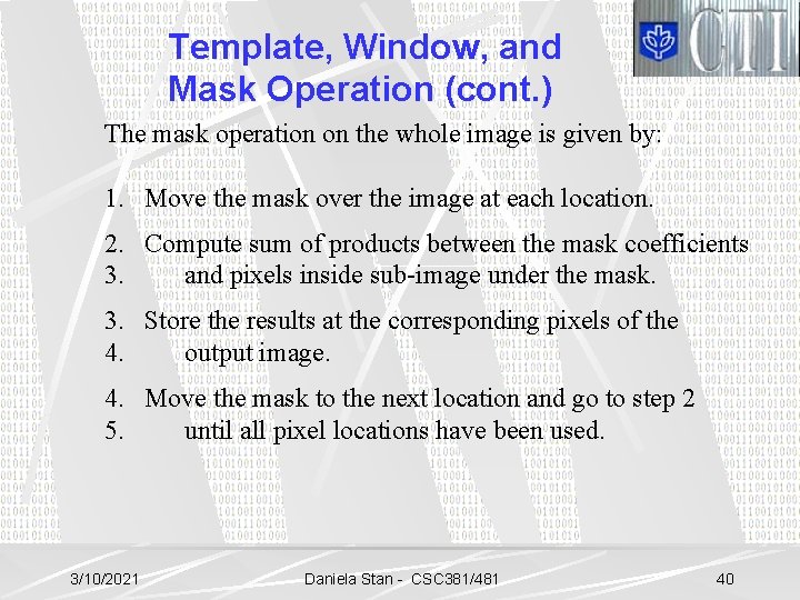
Template, Window, and Mask Operation (cont. ) The mask operation on the whole image is given by: 1. Move the mask over the image at each location. 2. Compute sum of products between the mask coefficients 3. and pixels inside sub-image under the mask. 3. Store the results at the corresponding pixels of the 4. output image. 4. Move the mask to the next location and go to step 2 5. until all pixel locations have been used. 3/10/2021 Daniela Stan - CSC 381/481 40

Template, Window, and Mask Operation (cont. ) Examples of the masks Sobel operators 3 x 3 moving average filter -1 0 -2 0 1 1 -1 -2 -1 0 0 0 -1 0 1 1 2 1 1 1 1 1 3 x 3 sharpening filter -1 -1 8 -1 -1 3/10/2021 Daniela Stan - CSC 381/481 41

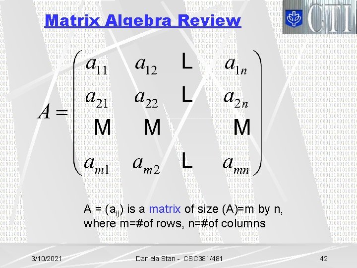
Matrix Algebra Review A = (aij) is a matrix of size (A)=m by n, where m=#of rows, n=#of columns 3/10/2021 Daniela Stan - CSC 381/481 42

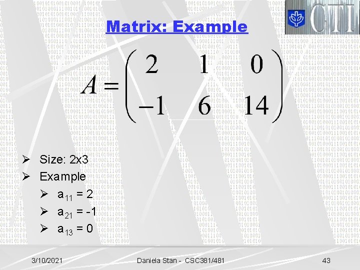
Matrix: Example Ø Size: 2 x 3 Ø Example Ø a 11 = 2 Ø a 21 = -1 Ø a 13 = 0 3/10/2021 Daniela Stan - CSC 381/481 43

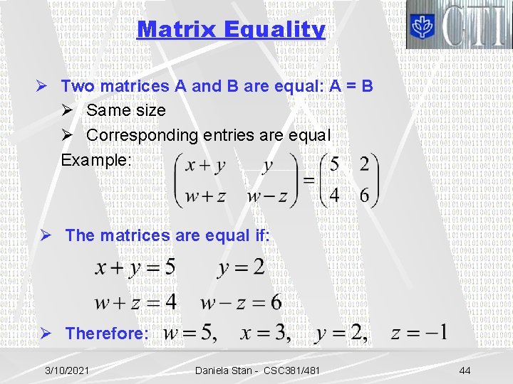
Matrix Equality Ø Two matrices A and B are equal: A = B Ø Same size Ø Corresponding entries are equal Example: Ø The matrices are equal if: Ø Therefore: 3/10/2021 Daniela Stan - CSC 381/481 44

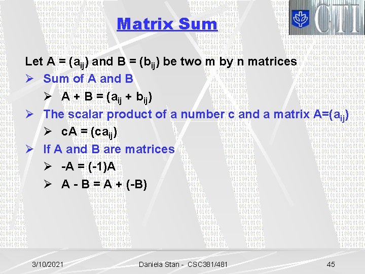
Matrix Sum Let A = (aij) and B = (bij) be two m by n matrices Ø Sum of A and B Ø A + B = (aij + bij) Ø The scalar product of a number c and a matrix A=(aij) Ø c. A = (caij) Ø If A and B are matrices Ø -A = (-1)A Ø A - B = A + (-B) 3/10/2021 Daniela Stan - CSC 381/481 45

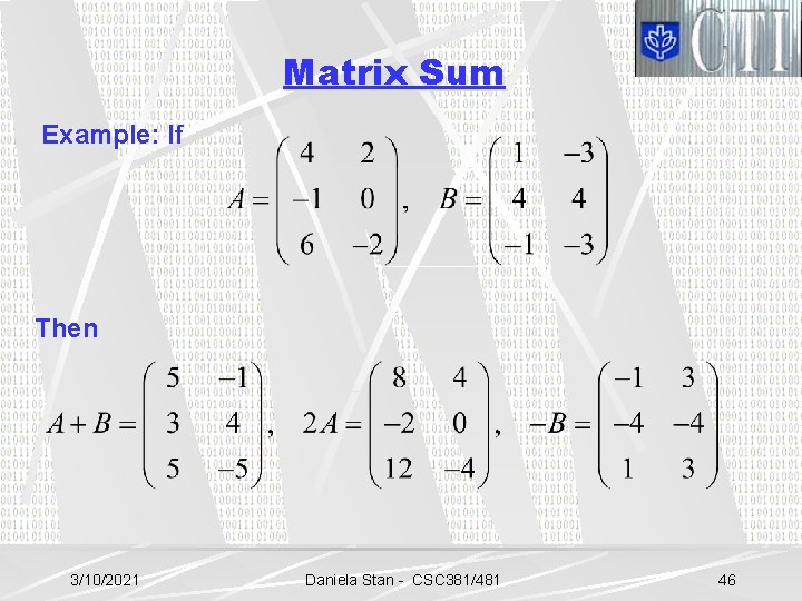
Matrix Sum Example: If Then 3/10/2021 Daniela Stan - CSC 381/481 46

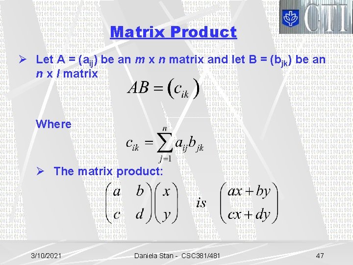
Matrix Product Ø Let A = (aij) be an m x n matrix and let B = (bjk) be an n x l matrix Where Ø The matrix product: 3/10/2021 Daniela Stan - CSC 381/481 47

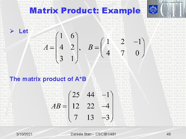
Matrix Product: Example Ø Let The matrix product of A*B 3/10/2021 Daniela Stan - CSC 381/481 48

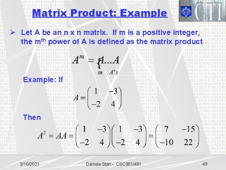
Matrix Product: Example Ø Let A be an n x n matrix. If m is a positive integer, the mth power of A is defined as the matrix product Example: If Then 3/10/2021 Daniela Stan - CSC 381/481 49

References Ø Lecture slides: Ø Textbook: Digital Image Processing by R. Gonzalez Ø Http: //gear. kku. ac. th/~nawapak/ip. html Ø Book: Discrete Mathematics by R. Johnsonbaugh 3/10/2021 Daniela Stan - CSC 381/481 50