CSC 323 Quarter Winter 0203 Daniela Stan Raicu

CSC 323 Quarter: Winter 02/03 Daniela Stan Raicu School of CTI, De. Paul University 12/12/2021 Daniela Stan - CSC 323 1

Outline • Describing distributions with numbers (continuation from the previous lecture) • The 1. 5 X IQR criterion for suspected outliers • Measuring spread: the standard deviation • Normal Distribution • Standard Normal Distribution 12/12/2021 Daniela Stan - CSC 323 2

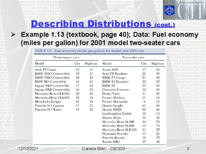
Describing Distributions (cont. ) Ø Example 1. 13 (textbook, page 40); Data: Fuel economy (miles per gallon) for 2001 model two-seater cars 12/12/2021 Daniela Stan - CSC 323 3

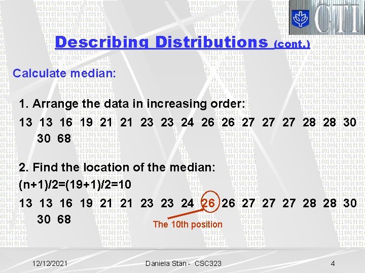
Describing Distributions (cont. ) Calculate median: 1. Arrange the data in increasing order: 13 13 16 19 21 21 23 23 24 26 26 27 27 27 28 28 30 30 68 2. Find the location of the median: (n+1)/2=(19+1)/2=10 13 13 16 19 21 21 23 23 24 26 26 27 27 27 28 28 30 30 68 The 10 th position 12/12/2021 Daniela Stan - CSC 323 4

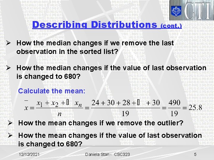
Describing Distributions (cont. ) Ø How the median changes if we remove the last observation in the sorted list? Ø How the median changes if the value of last observation is changed to 680? Calculate the mean: Ø How the mean changes if we remove the outlier? Ø How the mean changes if the value of last observation is changed to 680? 12/12/2021 Daniela Stan - CSC 323 5

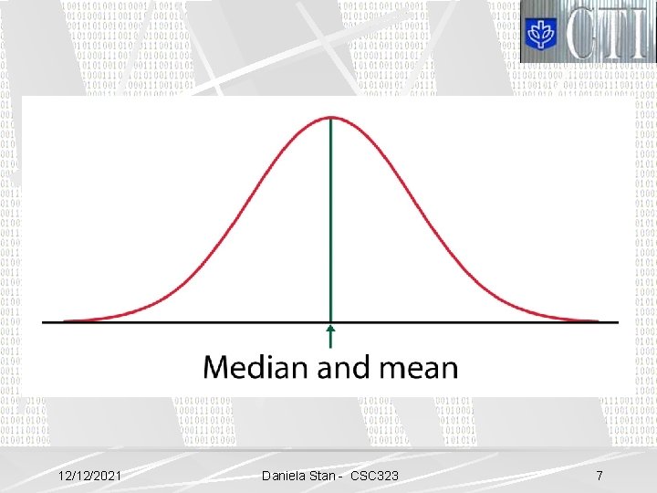
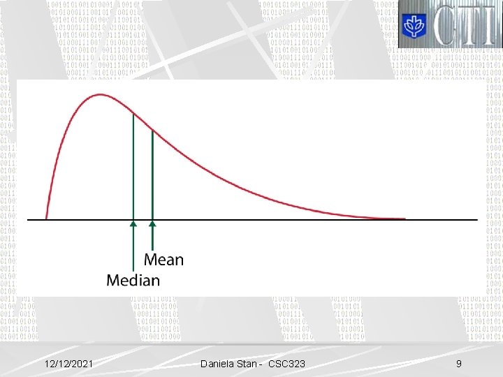
Describing Distributions (cont. ) Ø Mean versus Median 1. The mean is sensitive to the influence of extreme observations/outliers, or skewed distributions. 2. A resistant measure of any aspect of a distribution is relatively unaffected by changes in the numerical value of a small proportion of the total number of observations, no matter how large these changes are. 3. The mean is no a resistant measure of the center. 4. The median is a resistant measure of the center. 12/12/2021 Daniela Stan - CSC 323 6

12/12/2021 Daniela Stan - CSC 323 7

Median versus Average A recent newspaper article in California said that the median price of single-family homes sold in the past year in the local area was $136, 000 and the average price was $149, 160. How do you think these values are computed? Which do you think is more useful to someone considering the purchase of a home, the median or the average? 12/12/2021 Daniela Stan - CSC 323 8

12/12/2021 Daniela Stan - CSC 323 9

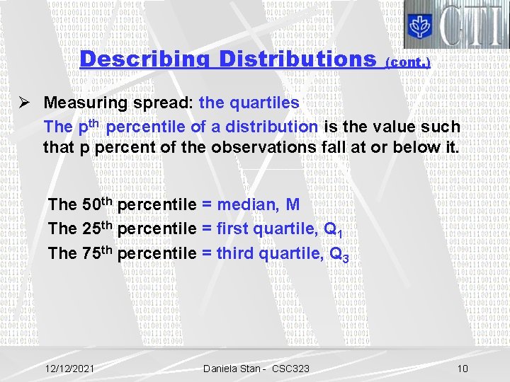
Describing Distributions (cont. ) Ø Measuring spread: the quartiles The pth percentile of a distribution is the value such that p percent of the observations fall at or below it. The 50 th percentile = median, M The 25 th percentile = first quartile, Q 1 The 75 th percentile = third quartile, Q 3 12/12/2021 Daniela Stan - CSC 323 10

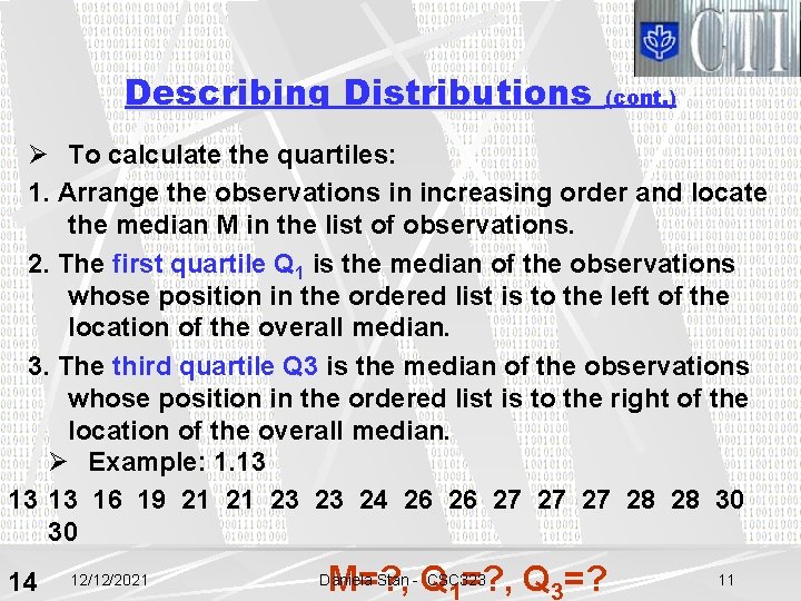
Describing Distributions (cont. ) Ø To calculate the quartiles: 1. Arrange the observations in increasing order and locate the median M in the list of observations. 2. The first quartile Q 1 is the median of the observations whose position in the ordered list is to the left of the location of the overall median. 3. The third quartile Q 3 is the median of the observations whose position in the ordered list is to the right of the location of the overall median. Ø Example: 1. 13 13 13 16 19 21 21 23 23 24 26 26 27 27 27 28 28 30 30 14 12/12/2021 M=? , Q 1=? , Q 3=? Daniela Stan - CSC 323 11

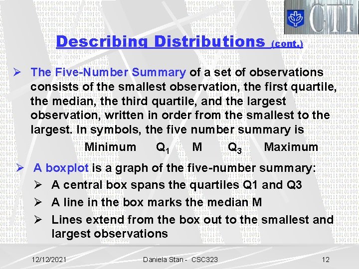
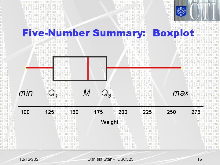
Describing Distributions (cont. ) Ø The Five-Number Summary of a set of observations consists of the smallest observation, the first quartile, the median, the third quartile, and the largest observation, written in order from the smallest to the largest. In symbols, the five number summary is Minimum Q 1 M Q 3 Maximum Ø A boxplot is a graph of the five-number summary: Ø A central box spans the quartiles Q 1 and Q 3 Ø A line in the box marks the median M Ø Lines extend from the box out to the smallest and largest observations 12/12/2021 Daniela Stan - CSC 323 12

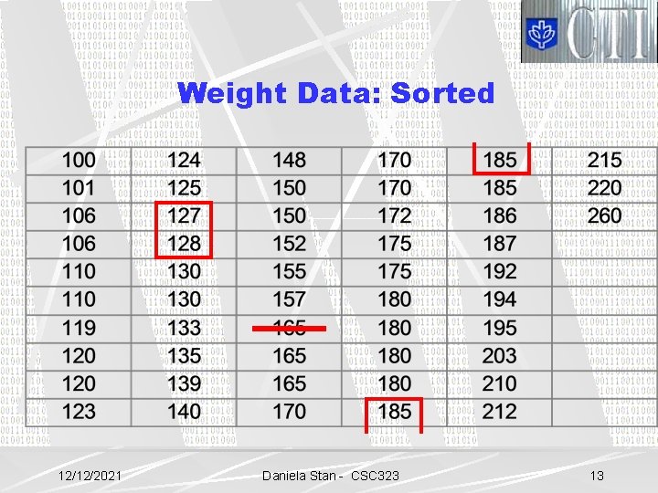
Weight Data: Sorted 12/12/2021 Daniela Stan - CSC 323 13

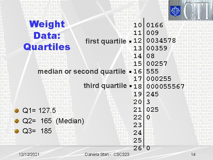
Weight Data: Quartiles 10 11 first quartile 12 13 14 15 median or second quartile 16 17 third quartile 18 19 20 21 Q 1= 127. 5 22 Q 2= 165 (Median) 23 Q 3= 185 24 25 26 12/12/2021 Daniela Stan - CSC 323 0166 009 0034578 00359 08 00257 555 000255 000055567 245 3 025 0 0 14

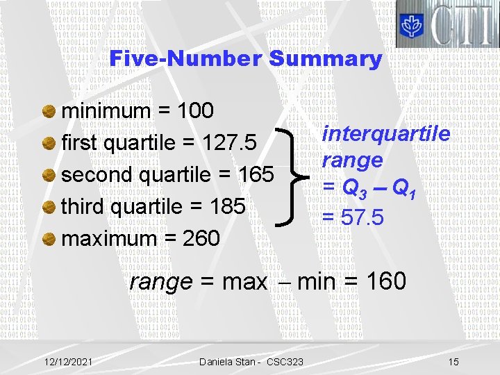
Five-Number Summary minimum = 100 first quartile = 127. 5 second quartile = 165 third quartile = 185 maximum = 260 interquartile range = Q 3 Q 1 = 57. 5 range = max min = 160 12/12/2021 Daniela Stan - CSC 323 15

Five-Number Summary: Boxplot min 100 Q 1 125 M 150 Q 3 175 max 200 225 250 275 Weight 12/12/2021 Daniela Stan - CSC 323 16

Recommended Problems Ø Chapter 1: Section 1. 1 Problems 1. 14, 1. 15, 1. 16, 1. 20, 1. 23, 1. 26, 1. 34 Ø Chapter 1: Section 1. 2 Problems 1. 46, 1. 48 Ø IPS web site: http: //www. whfreeman. com/ips 4 e 12/12/2021 Daniela Stan - CSC 323 17

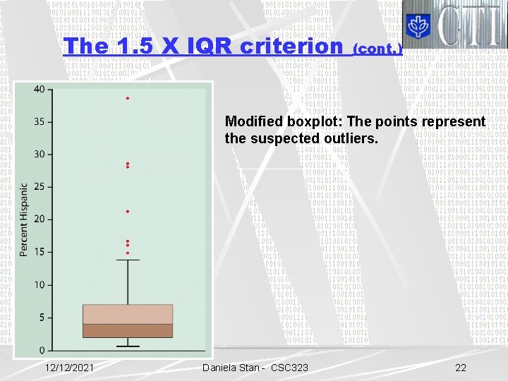
The 1. 5 X IQR criterion Ø The interquartile range IQR: is the distance between the first and third quartiles: IQR=Q 3 – Q 1 Ø The 1. 5 X IQR criterion for outliers: An observation is a suspect outlier if it falls more than 1. 5 X IQR above third quartile or below the first quartile. Ø Modified boxplot: - the lines extend out from the central box only to the smallest and largest observations that are not suspected outliers. - the suspected outliers are plotted as individual points. 12/12/2021 Daniela Stan - CSC 323 18

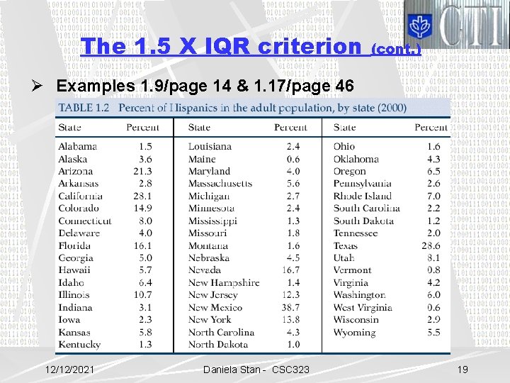
The 1. 5 X IQR criterion (cont. ) Ø Examples 1. 9/page 14 & 1. 17/page 46 12/12/2021 Daniela Stan - CSC 323 19

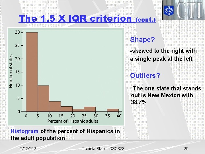
The 1. 5 X IQR criterion (cont. ) Shape? -skewed to the right with a single peak at the left Outliers? -The one state that stands out is New Mexico with 38. 7% Histogram of the percent of Hispanics in the adult population 12/12/2021 Daniela Stan - CSC 323 20

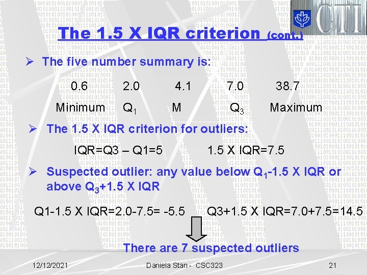
The 1. 5 X IQR criterion (cont. ) Ø The five number summary is: 0. 6 2. 0 4. 1 7. 0 Minimum Q 1 M Q 3 38. 7 Maximum Ø The 1. 5 X IQR criterion for outliers: IQR=Q 3 – Q 1=5 1. 5 X IQR=7. 5 Ø Suspected outlier: any value below Q 1 -1. 5 X IQR or above Q 3+1. 5 X IQR Q 1 -1. 5 X IQR=2. 0 -7. 5= -5. 5 Q 3+1. 5 X IQR=7. 0+7. 5=14. 5 There are 7 suspected outliers 12/12/2021 Daniela Stan - CSC 323 21

The 1. 5 X IQR criterion (cont. ) Modified boxplot: The points represent the suspected outliers. 12/12/2021 Daniela Stan - CSC 323 22

Measuring the spread: Variance and Standard Deviation If all values are the same, what is the variation in the data? Variation exists when some values are above or below the mean. Each data value has an associated deviation from the mean 12/12/2021 Daniela Stan - CSC 323 23

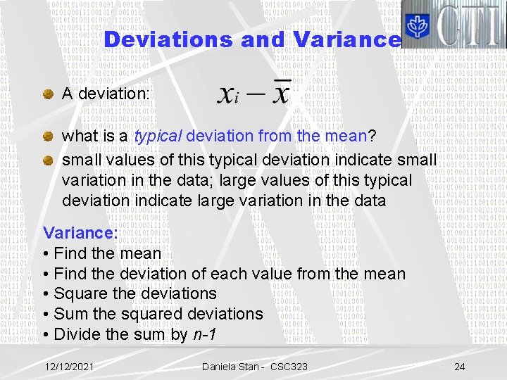
Deviations and Variance A deviation: what is a typical deviation from the mean? small values of this typical deviation indicate small variation in the data; large values of this typical deviation indicate large variation in the data Variance: • Find the mean • Find the deviation of each value from the mean • Square the deviations • Sum the squared deviations • Divide the sum by n-1 12/12/2021 Daniela Stan - CSC 323 24

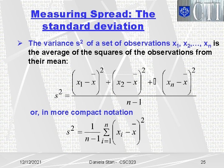
Measuring Spread: The standard deviation Ø The variance s 2 of a set of observations x 1, x 2, …, xn is the average of the squares of the observations from their mean: or, in more compact notation 12/12/2021 Daniela Stan - CSC 323 25

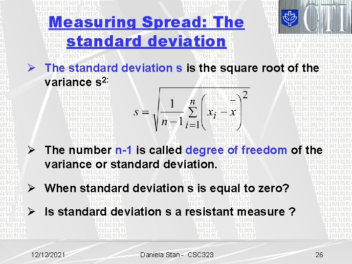
Measuring Spread: The standard deviation Ø The standard deviation s is the square root of the variance s 2: Ø The number n-1 is called degree of freedom of the variance or standard deviation. Ø When standard deviation s is equal to zero? Ø Is standard deviation s a resistant measure ? 12/12/2021 Daniela Stan - CSC 323 26

The standard deviation (cont. ) Ø Example: Ø Problem 1. 59 Ø Choosing measures for center and spread: - if the distribution is skewed, choose five number summary - if the distribution is symmetric and free of outliers, choose the mean and the standard deviation 12/12/2021 Daniela Stan - CSC 323 27

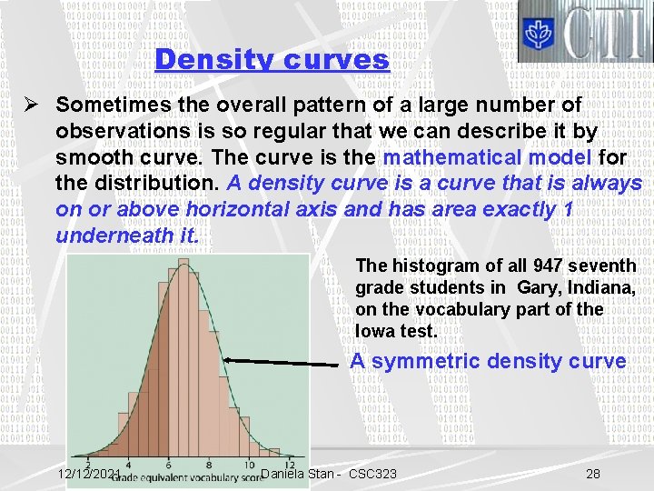
Density curves Ø Sometimes the overall pattern of a large number of observations is so regular that we can describe it by smooth curve. The curve is the mathematical model for the distribution. A density curve is a curve that is always on or above horizontal axis and has area exactly 1 underneath it. The histogram of all 947 seventh grade students in Gary, Indiana, on the vocabulary part of the Iowa test. A symmetric density curve 12/12/2021 Daniela Stan - CSC 323 28

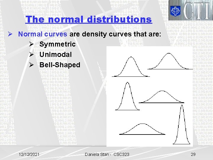
The normal distributions Ø Normal curves are density curves that are: Ø Symmetric Ø Unimodal Ø Bell-Shaped 12/12/2021 Daniela Stan - CSC 323 29

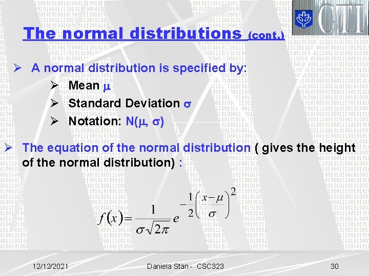
The normal distributions (cont. ) Ø A normal distribution is specified by: Ø Mean Ø Standard Deviation Ø Notation: N( , ) Ø The equation of the normal distribution ( gives the height of the normal distribution) : 12/12/2021 Daniela Stan - CSC 323 30

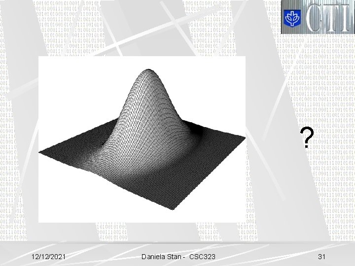
? 12/12/2021 Daniela Stan - CSC 323 31

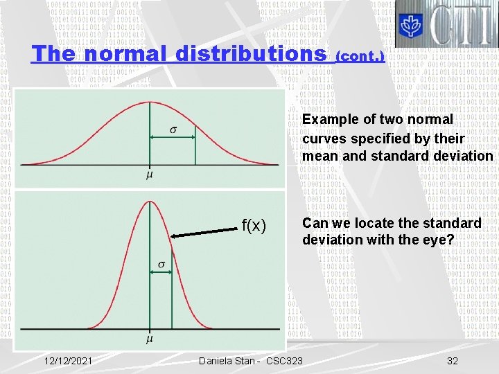
The normal distributions (cont. ) Example of two normal curves specified by their mean and standard deviation f(x) 12/12/2021 Can we locate the standard deviation with the eye? Daniela Stan - CSC 323 32

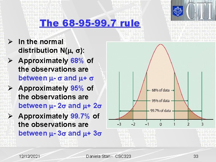
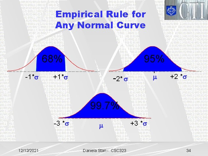
The 68 -95 -99. 7 rule Ø In the normal distribution N( , ): Ø Approximately 68% of the observations are between - and + Ø Approximately 95% of the observations are between - 2 and + 2 Ø Approximately 99. 7% of the observations are between - 3 and + 3 12/12/2021 Daniela Stan - CSC 323 33

Empirical Rule for Any Normal Curve 68% -1* 95% -2* +1* +2 * 99. 7% -3 * 12/12/2021 Daniela Stan - CSC 323 +3 * 34

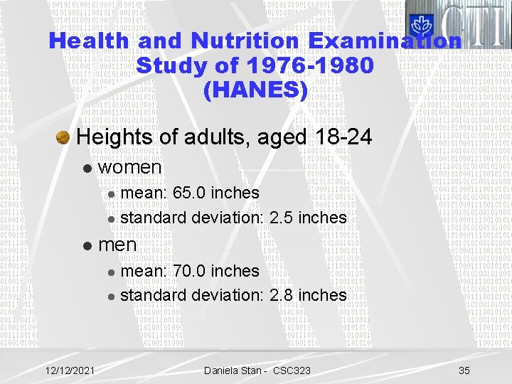
Health and Nutrition Examination Study of 1976 -1980 (HANES) Heights of adults, aged 18 -24 l women mean: 65. 0 inches l standard deviation: 2. 5 inches l l men mean: 70. 0 inches l standard deviation: 2. 8 inches l 12/12/2021 Daniela Stan - CSC 323 35

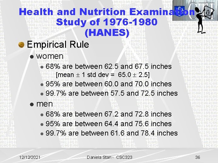
Health and Nutrition Examination Study of 1976 -1980 (HANES) Empirical Rule l women l 68% are between 62. 5 and 67. 5 inches [mean 1 std dev = 65. 0 2. 5] 95% are between 60. 0 and 70. 0 inches l 99. 7% are between 57. 5 and 72. 5 inches l l men 68% are between 67. 2 and 72. 8 inches l 95% are between 64. 4 and 75. 6 inches l 99. 7% are between 61. 6 and 78. 4 inches l 12/12/2021 Daniela Stan - CSC 323 36

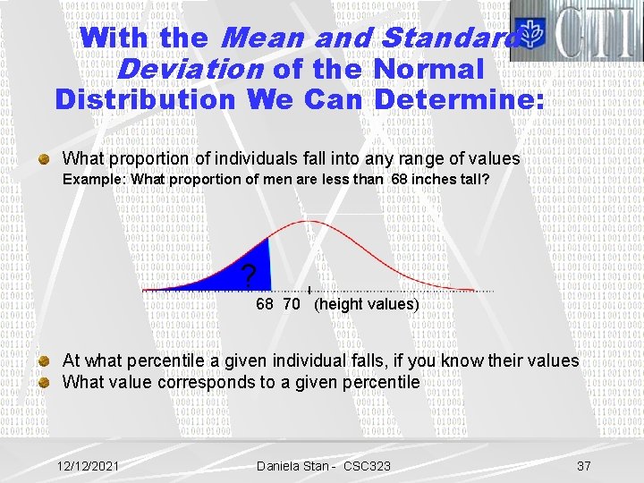
With the Mean and Standard Deviation of the Normal Distribution We Can Determine: What proportion of individuals fall into any range of values Example: What proportion of men are less than 68 inches tall? ? 68 70 (height values) At what percentile a given individual falls, if you know their values What value corresponds to a given percentile 12/12/2021 Daniela Stan - CSC 323 37

Health and Nutrition Examination Study of 1976 -1980 (HANES) The answer is given in the next lecture using standard normal distributions. 12/12/2021 Daniela Stan - CSC 323 38