CSC 321 Tutorial with extra material on Semantic

CSC 321: Tutorial with extra material on: Semantic Hashing and Conditional Restricted Boltzmann Machines (This will not be in the final exam) Geoffrey Hinton

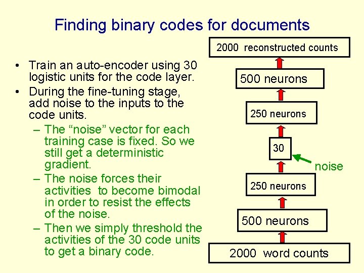
Finding binary codes for documents 2000 reconstructed counts • Train an auto-encoder using 30 logistic units for the code layer. • During the fine-tuning stage, add noise to the inputs to the code units. – The “noise” vector for each training case is fixed. So we still get a deterministic gradient. – The noise forces their activities to become bimodal in order to resist the effects of the noise. – Then we simply threshold the activities of the 30 code units to get a binary code. 500 neurons 250 neurons 30 noise 250 neurons 500 neurons 2000 word counts

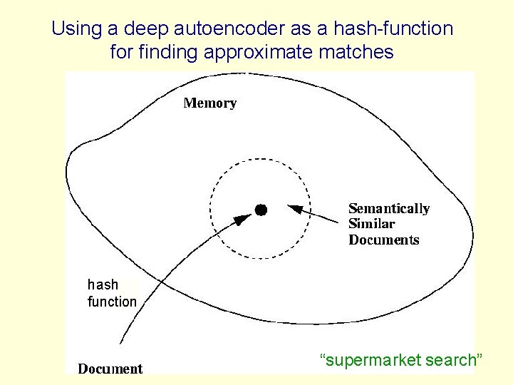
Using a deep autoencoder as a hash-function for finding approximate matches hash function “supermarket search”

Another view of semantic hashing • Fast retrieval methods typically work by intersecting stored lists that are associated with cues extracted from the query. • Computers have special hardware that can intersect 32 very long lists in one instruction. – Each bit in a 32 -bit binary code specifies a list of half the addresses in the memory. • Semantic hashing uses machine learning to map the retrieval problem onto the type of list intersection the computer is good at.

How good is a shortlist found this way? • Russ has only implemented it for a million documents with 20 -bit codes --- but what could possibly go wrong? – A 20 -D hypercube allows us to capture enough of the similarity structure of our document set. • The shortlist found using binary codes actually improves the precision-recall curves of TF-IDF. – Locality sensitive hashing (the fastest other method) is much slower and has worse precision-recall curves.

Semantic hashing for image retrieval • Currently, image retrieval is typically done by using the captions. Why not use the images too? – Pixels are not like words: individual pixels do not tell us much about the content. – Extracting object classes from images is hard. • Maybe we should extract a real-valued vector that has information about the content? – Matching real-valued vectors in a big database is slow and requires a lot of storage • Short binary codes are easy to store and match

A two-stage method • First, use semantic hashing with 28 -bit binary codes to get a long “shortlist” of promising images. • Then use 256 -bit binary codes to do a serial search for good matches. – This only requires a few words of storage per image and the serial search can be done using fast bit-operations. • But how good are the 256 -bit binary codes? – Do they find images that we think are similar?

Some depressing competition • Inspired by the speed of semantic hashing, Weiss, Fergus and Torralba (NIPS 2008) used a very fast spectral method to assign binary codes to images. – This eliminates the long learning times required by deep autoencoders. • They claimed that their spectral method gave better retrieval results than training a deep auto-encoder using RBM’s. – But they could not get RBM’s to work well for extracting features from RGB pixels so they started from 384 GIST features. – This is too much dimensionality reduction too soon.

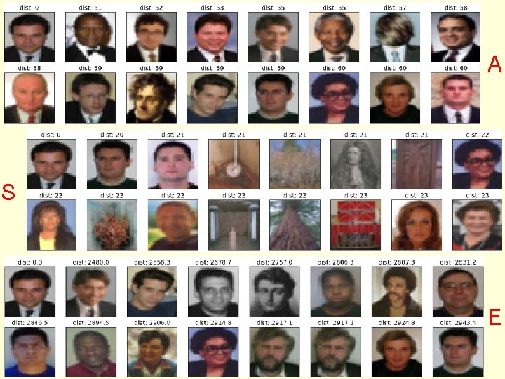
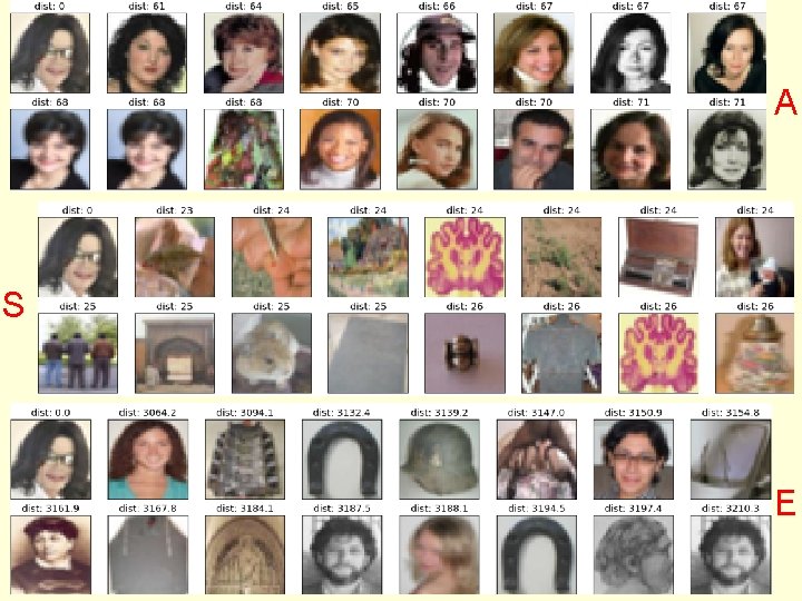
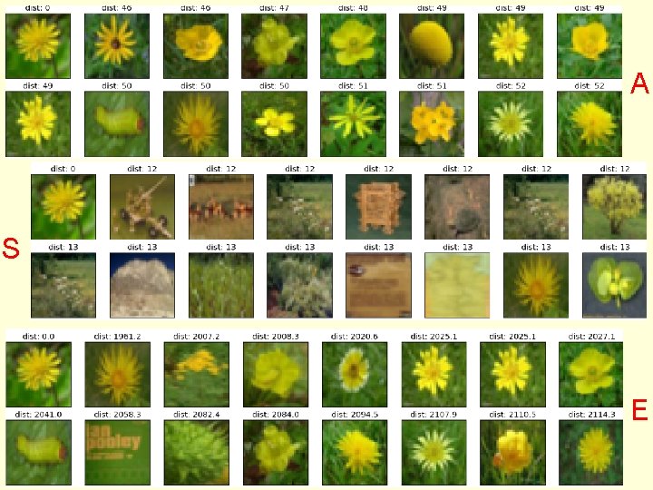
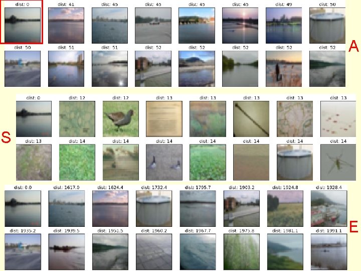
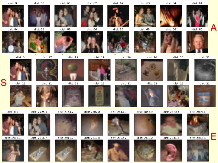
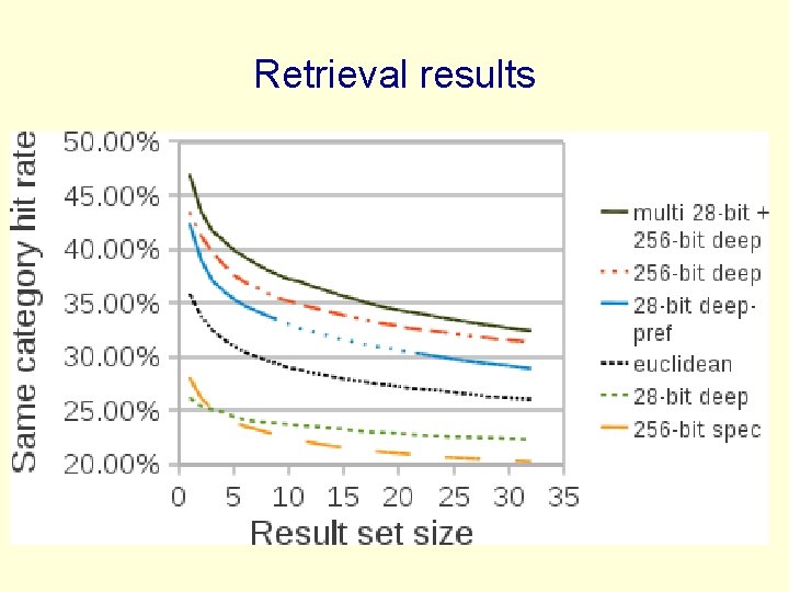
A comparison of deep auto-encoders and the spectral method using 256 -bit codes (Alex Krizhevsky) • Train auto-encoders “properly” – Use Gaussian visible units with fixed variance. Do not add noise to the reconstructions. – Use a cluster machine or a big GPU board. – Use a lot of hidden units in the early layers. • Then compare with the spectral method – The spectral method has no free parameters. • Also compare with Euclidean match in pixel space

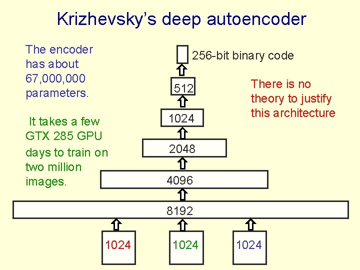
Krizhevsky’s deep autoencoder The encoder has about 67, 000 parameters. 256 -bit binary code 512 It takes a few GTX 285 GPU days to train on two million images. 1024 There is no theory to justify this architecture 2048 4096 8192 1024

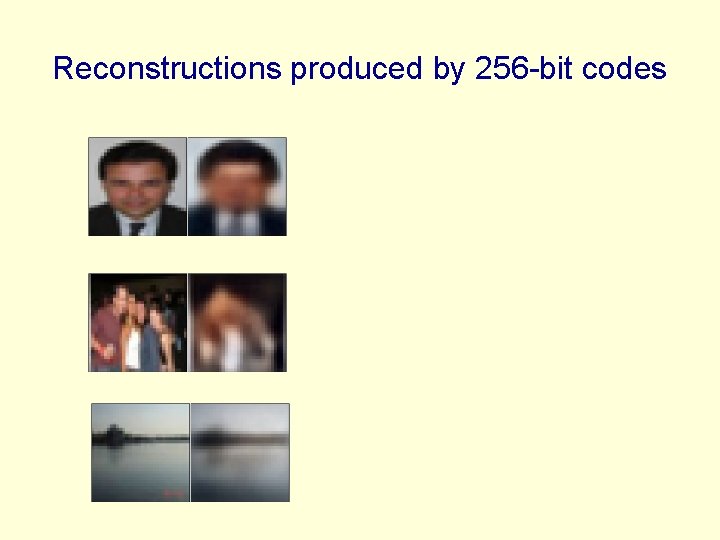
Reconstructions produced by 256 -bit codes

A S E

A S E

A S E

A S E

A S E

Retrieval results

An obvious extension • Use a multimedia auto-encoder that represents captions and images in a single code. – The captions should help it extract more meaningful image features such as “contains an animal” or “indoor image” • RBM’s already work much better than standard LDA topic models for modeling bags of words. – So the multimedia auto-encoder should be a win (for images) a win (for captions) a win (for the interaction during training)

A less obvious extension • Semantic hashing gives incredibly fast retrieval but its hard to go much beyond 32 bits. • We can afford to use semantic hashing several times with variations of the query and merge the shortlists – Its easy to enumerate the hamming ball around a query image address in ascending address order, so merging is linear time. • Apply many transformations to the query image to get transformation independent retrieval. – Image translations are an obvious candidate.

A more interesting extension • Computer vision uses images of uniform resolution. – Multi-resolution images still keep all the highresolution pixels. • Even on 32 x 32 images, people use a lot of eye movements to attend to different parts of the image. – Human vision copes with big translations by moving the fixation point. – It only samples a tiny fraction of the image at high resolution. The “post-retinal’’ image has resolution that falls off rapidly outside the fovea. – With less “neurons” intelligent sampling becomes even more important.

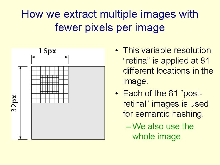
How we extract multiple images with fewer pixels per image • This variable resolution “retina” is applied at 81 different locations in the image. • Each of the 81 “postretinal” images is used for semantic hashing. – We also use the whole image.

A more human metric for image similarity • Two images are similar if fixating at point X in one image and point Y in the other image gives similar post-retinal images. • So use semantic hashing on post-retinal images. – The address space is used for post-retinal images and each address points to the whole image that the post-retinal image came from. – So we can accumulate similarity over multiple fixations. • The whole image addresses found after each fixation have to be sorted to allow merging

Summary • Restricted Boltzmann Machines provide an efficient way to learn a layer of features without any supervision. – Many layers of representation can be learned by treating the hidden states of one RBM as the data for the next. • This allows us to learn very deep nets that extract short binary codes for unlabeled images or documents. – Using 32 -bit codes as addresses allows us to get approximate matches at the speed of hashing. • Semantic hashing is fast enough to allow many retrieval cycles for a single query image. – So we can try multiple transformations of the query.

Time series models • Inference is difficult in directed models of time series if we use non-linear distributed representations in the hidden units. – It is hard to fit Dynamic Bayes Nets to highdimensional sequences (e. g motion capture data). • So people tend to avoid distributed representations and use much weaker methods (e. g. HMM’s).

Time series models • If we really need distributed representations (which we nearly always do), we can make inference much simpler by using three tricks: – Use an RBM for the interactions between hidden and visible variables. This ensures that the main source of information wants the posterior to be factorial. – Model short-range temporal information by allowing several previous frames to provide input to the hidden units and to the visible units. • This leads to a temporal module that can be stacked – So we can use greedy learning to learn deep models of temporal structure.

An application to modeling motion capture data (Taylor, Roweis & Hinton, 2007) • Human motion can be captured by placing reflective markers on the joints and then using lots of infrared cameras to track the 3 -D positions of the markers. • Given a skeletal model, the 3 -D positions of the markers can be converted into the joint angles plus 6 parameters that describe the 3 -D position and the roll, pitch and yaw of the pelvis. – We only represent changes in yaw because physics doesn’t care about its value and we want to avoid circular variables.

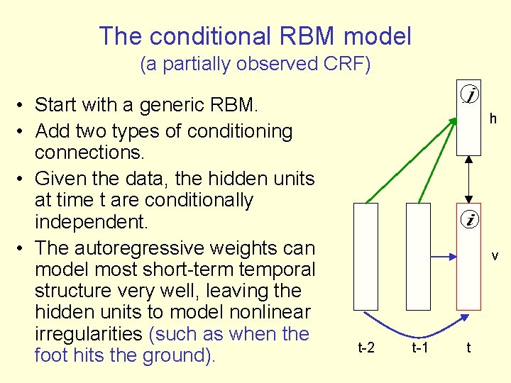
The conditional RBM model (a partially observed CRF) • Start with a generic RBM. • Add two types of conditioning connections. • Given the data, the hidden units at time t are conditionally independent. • The autoregressive weights can model most short-term temporal structure very well, leaving the hidden units to model nonlinear irregularities (such as when the foot hits the ground). h v t-2 t-1 t

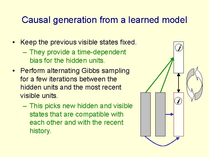
Causal generation from a learned model • Keep the previous visible states fixed. – They provide a time-dependent bias for the hidden units. • Perform alternating Gibbs sampling for a few iterations between the hidden units and the most recent visible units. – This picks new hidden and visible states that are compatible with each other and with the recent history.

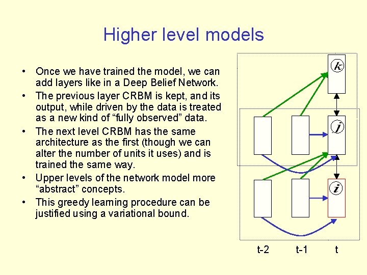
Higher level models • Once we have trained the model, we can add layers like in a Deep Belief Network. • The previous layer CRBM is kept, and its output, while driven by the data is treated as a new kind of “fully observed” data. • The next level CRBM has the same architecture as the first (though we can alter the number of units it uses) and is trained the same way. • Upper levels of the network model more “abstract” concepts. • This greedy learning procedure can be justified using a variational bound. t-2 t-1 t

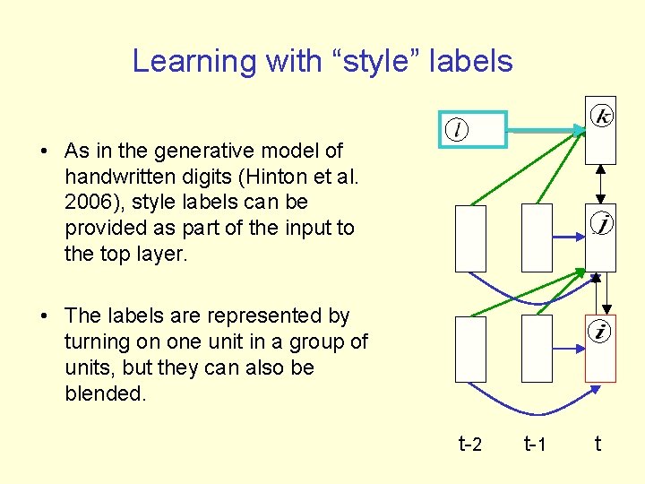
Learning with “style” labels • As in the generative model of handwritten digits (Hinton et al. 2006), style labels can be provided as part of the input to the top layer. • The labels are represented by turning on one unit in a group of units, but they can also be blended. t-2 t-1 t

Show demo’s of multiple styles of walking These can be found at www. cs. toronto. edu/~gwtaylor/