CS 252 Graduate Computer Architecture Lecture 22 Memory

CS 252 Graduate Computer Architecture Lecture 22 Memory Technology Error Correction Codes April 16 th, 2012 John Kubiatowicz Electrical Engineering and Computer Sciences University of California, Berkeley http: //www. eecs. berkeley. edu/~kubitron/cs 252

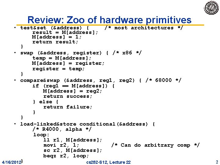
Review: Zoo of hardware primitives • test&set (&address) { /* most architectures */ result = M[address]; M[address] = 1; return result; } • swap (&address, register) { /* x 86 */ temp = M[address]; M[address] = register; register = temp; } • compare&swap (&address, reg 1, reg 2) { /* 68000 */ if (reg 1 == M[address]) { M[address] = reg 2; return success; } else { return failure; } } • load-linked&store conditional(&address) { /* R 4000, alpha */ loop: ll r 1, M[address]; movi r 2, 1; /* Can do arbitrary comp */ sc r 2, M[address]; beqz r 2, loop; 4/16/2012} cs 252 S 12, Lecture 22 2

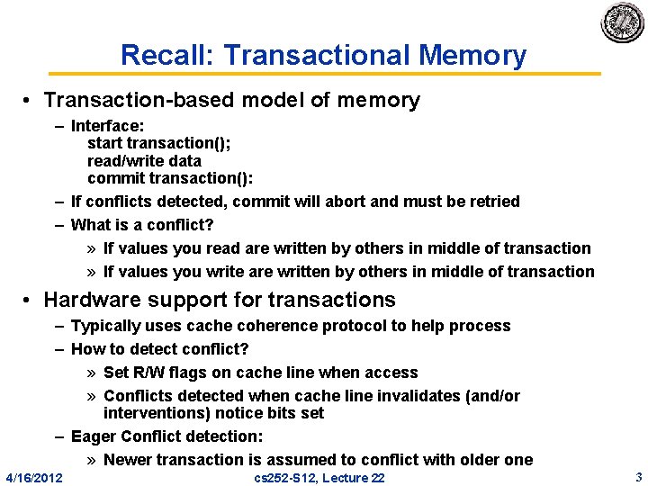
Recall: Transactional Memory • Transaction based model of memory – Interface: start transaction(); read/write data commit transaction(): – If conflicts detected, commit will abort and must be retried – What is a conflict? » If values you read are written by others in middle of transaction » If values you write are written by others in middle of transaction • Hardware support for transactions – Typically uses cache coherence protocol to help process – How to detect conflict? » Set R/W flags on cache line when access » Conflicts detected when cache line invalidates (and/or interventions) notice bits set – Eager Conflict detection: » Newer transaction is assumed to conflict with older one 4/16/2012 cs 252 S 12, Lecture 22 3

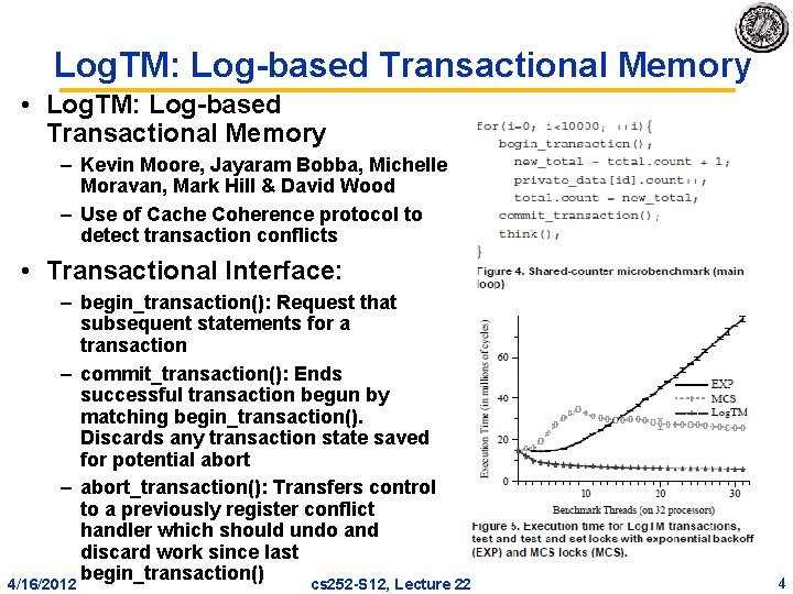
Log. TM: Log based Transactional Memory • Log. TM: Log based Transactional Memory – Kevin Moore, Jayaram Bobba, Michelle Moravan, Mark Hill & David Wood – Use of Cache Coherence protocol to detect transaction conflicts • Transactional Interface: – begin_transaction(): Request that subsequent statements for a transaction – commit_transaction(): Ends successful transaction begun by matching begin_transaction(). Discards any transaction state saved for potential abort – abort_transaction(): Transfers control to a previously register conflict handler which should undo and discard work since last begin_transaction() 4/16/2012 cs 252 S 12, Lecture 22 4

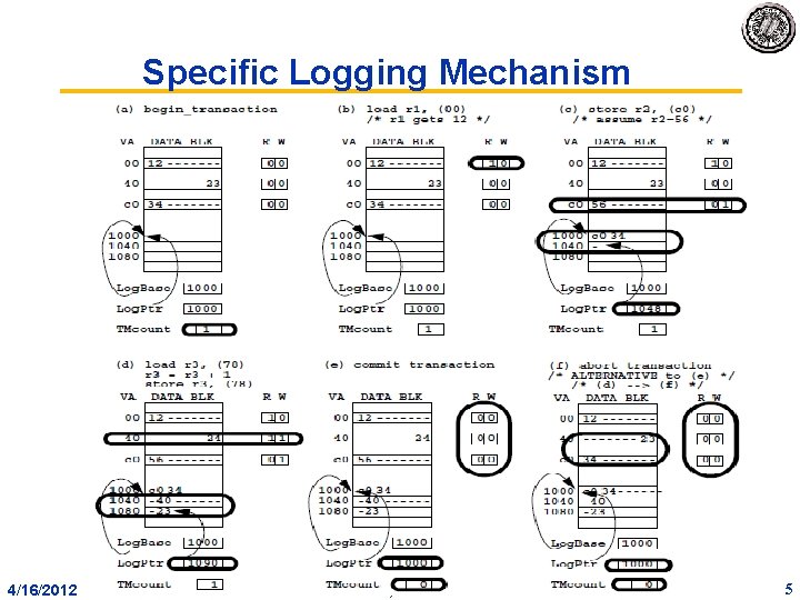
Specific Logging Mechanism 4/16/2012 cs 252 S 12, Lecture 22 5

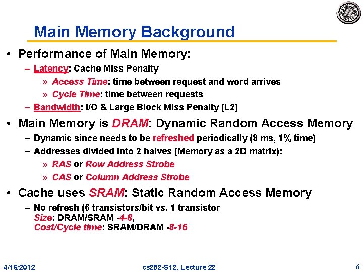
Main Memory Background • Performance of Main Memory: – Latency: Cache Miss Penalty » Access Time: time between request and word arrives » Cycle Time: time between requests – Bandwidth: I/O & Large Block Miss Penalty (L 2) • Main Memory is DRAM: Dynamic Random Access Memory – Dynamic since needs to be refreshed periodically (8 ms, 1% time) – Addresses divided into 2 halves (Memory as a 2 D matrix): » RAS or Row Address Strobe » CAS or Column Address Strobe • Cache uses SRAM: Static Random Access Memory – No refresh (6 transistors/bit vs. 1 transistor Size: DRAM/SRAM 4 -8, Cost/Cycle time: SRAM/DRAM 8 -16 4/16/2012 cs 252 S 12, Lecture 22 6

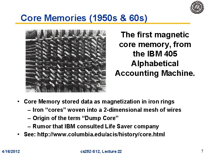
Core Memories (1950 s & 60 s) The first magnetic core memory, from the IBM 405 Alphabetical Accounting Machine. • Core Memory stored data as magnetization in iron rings – Iron “cores” woven into a 2 dimensional mesh of wires – Origin of the term “Dump Core” – Rumor that IBM consulted Life Saver company • See: http: //www. columbia. edu/acis/history/core. html 4/16/2012 cs 252 S 12, Lecture 22 7

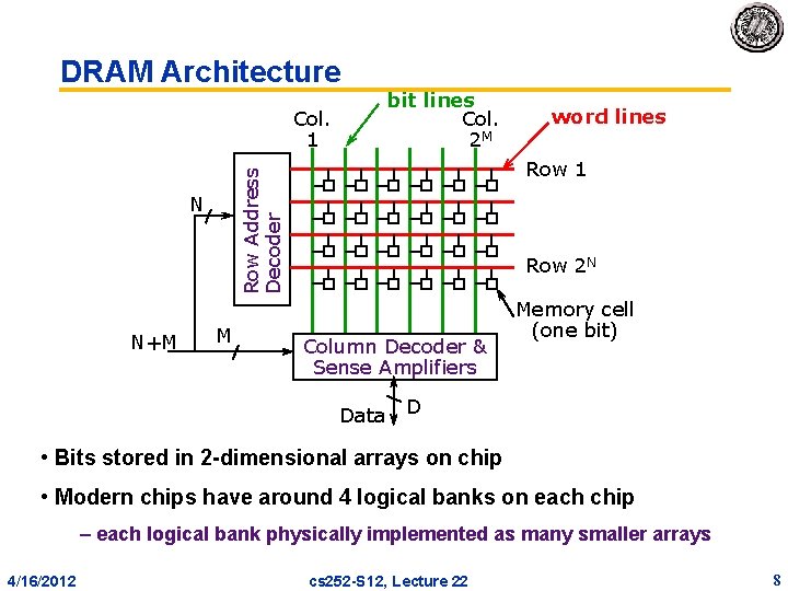
DRAM Architecture Col. 1 M word lines Row 1 Row Address Decoder N N+M bit lines Col. 2 M Row 2 N Column Decoder & Sense Amplifiers Data Memory cell (one bit) D • Bits stored in 2 dimensional arrays on chip • Modern chips have around 4 logical banks on each chip – each logical bank physically implemented as many smaller arrays 4/16/2012 cs 252 S 12, Lecture 22 8

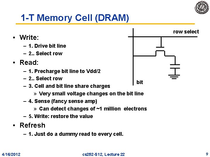
1 T Memory Cell (DRAM) row select • Write: – 1. Drive bit line – 2. . Select row • Read: – 1. Precharge bit line to Vdd/2 – 2. . Select row bit – 3. Cell and bit line share charges » Very small voltage changes on the bit line – 4. Sense (fancy sense amp) » Can detect changes of ~1 million electrons – 5. Write: restore the value • Refresh – 1. Just do a dummy read to every cell. 4/16/2012 cs 252 S 12, Lecture 22 9

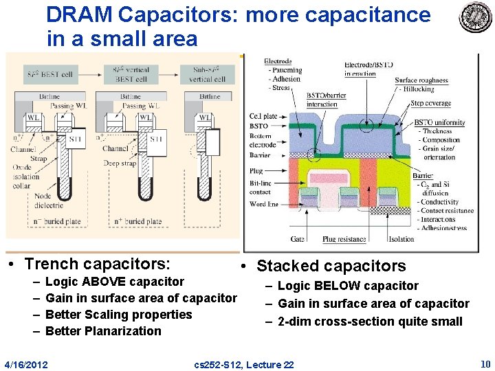
DRAM Capacitors: more capacitance in a small area • Trench capacitors: – – Logic ABOVE capacitor Gain in surface area of capacitor Better Scaling properties Better Planarization 4/16/2012 • Stacked capacitors – Logic BELOW capacitor – Gain in surface area of capacitor – 2 dim cross section quite small cs 252 S 12, Lecture 22 10

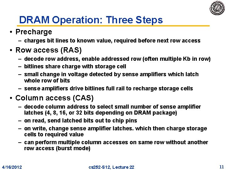
DRAM Operation: Three Steps • Precharge – charges bit lines to known value, required before next row access • Row access (RAS) – decode row address, enable addressed row (often multiple Kb in row) – bitlines share charge with storage cell – small change in voltage detected by sense amplifiers which latch whole row of bits – sense amplifiers drive bitlines full rail to recharge storage cells • Column access (CAS) – decode column address to select small number of sense amplifier latches (4, 8, 16, or 32 bits depending on DRAM package) – on read, send latched bits out to chip pins – on write, change sense amplifier latches. which then charge storage cells to required value – can perform multiple column accesses on same row without another row access (burst mode) 4/16/2012 cs 252 S 12, Lecture 22 11

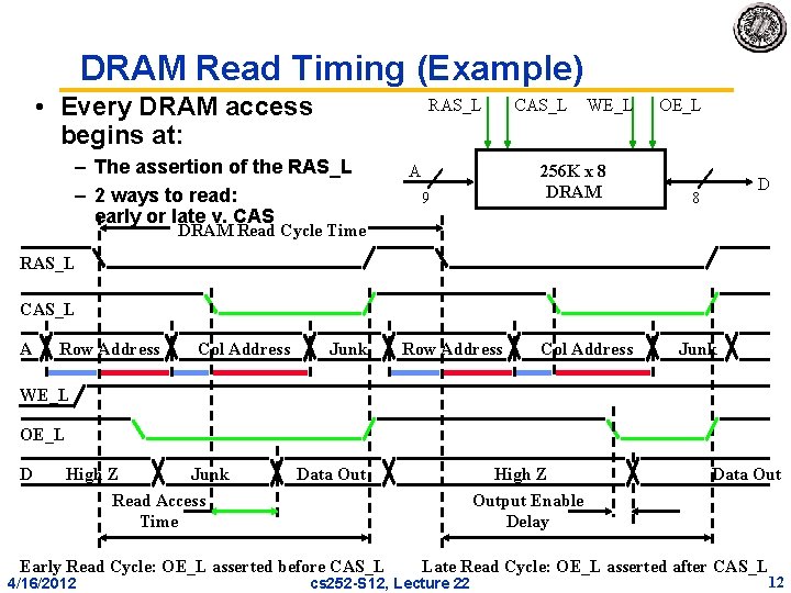
DRAM Read Timing (Example) • Every DRAM access begins at: RAS_L – The assertion of the RAS_L – 2 ways to read: early or late v. CAS_L WE_L 256 K x 8 DRAM A 9 OE_L D 8 DRAM Read Cycle Time RAS_L CAS_L A Row Address Col Address Junk WE_L OE_L D High Z Junk Read Access Time Data Out Early Read Cycle: OE_L asserted before CAS_L 4/16/2012 High Z Output Enable Delay Data Out Late Read Cycle: OE_L asserted after CAS_L cs 252 S 12, Lecture 22 12

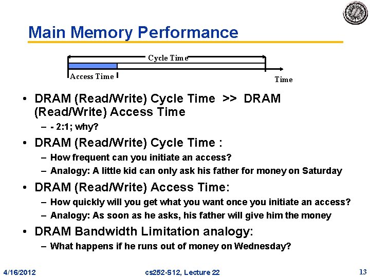
Main Memory Performance Cycle Time Access Time • DRAM (Read/Write) Cycle Time >> DRAM (Read/Write) Access Time – 2: 1; why? • DRAM (Read/Write) Cycle Time : – How frequent can you initiate an access? – Analogy: A little kid can only ask his father for money on Saturday • DRAM (Read/Write) Access Time: – How quickly will you get what you want once you initiate an access? – Analogy: As soon as he asks, his father will give him the money • DRAM Bandwidth Limitation analogy: – What happens if he runs out of money on Wednesday? 4/16/2012 cs 252 S 12, Lecture 22 13

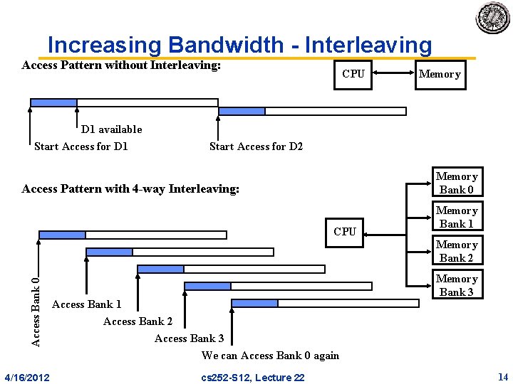
Increasing Bandwidth Interleaving Access Pattern without Interleaving: D 1 available Start Access for D 1 CPU Memory Start Access for D 2 Memory Bank 0 Access Pattern with 4 -way Interleaving: CPU Memory Bank 1 Access Bank 0 Memory Bank 2 4/16/2012 Access Bank 1 Access Bank 2 Access Bank 3 We can Access Bank 0 again cs 252 S 12, Lecture 22 Memory Bank 3 14

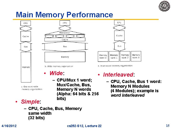
Main Memory Performance • Wide: • Simple: • Interleaved: – CPU/Mux 1 word; Mux/Cache, Bus, Memory N words (Alpha: 64 bits & 256 bits) – CPU, Cache, Bus 1 word: Memory N Modules (4 Modules); example is word interleaved – CPU, Cache, Bus, Memory same width (32 bits) 4/16/2012 cs 252 S 12, Lecture 22 15

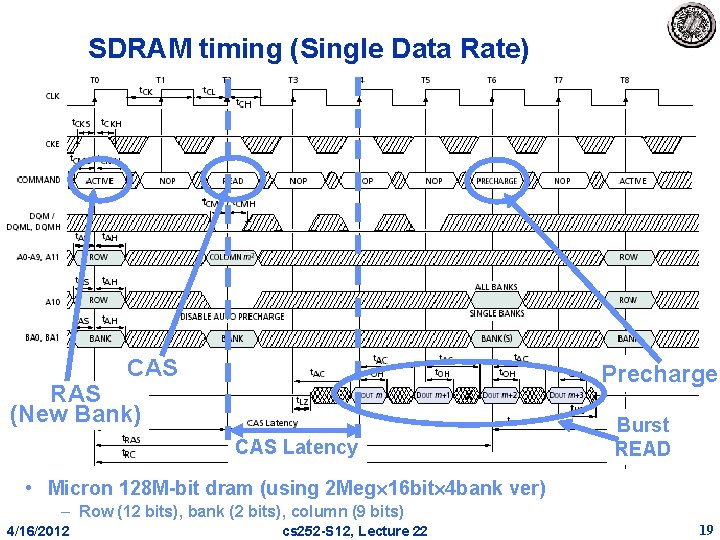
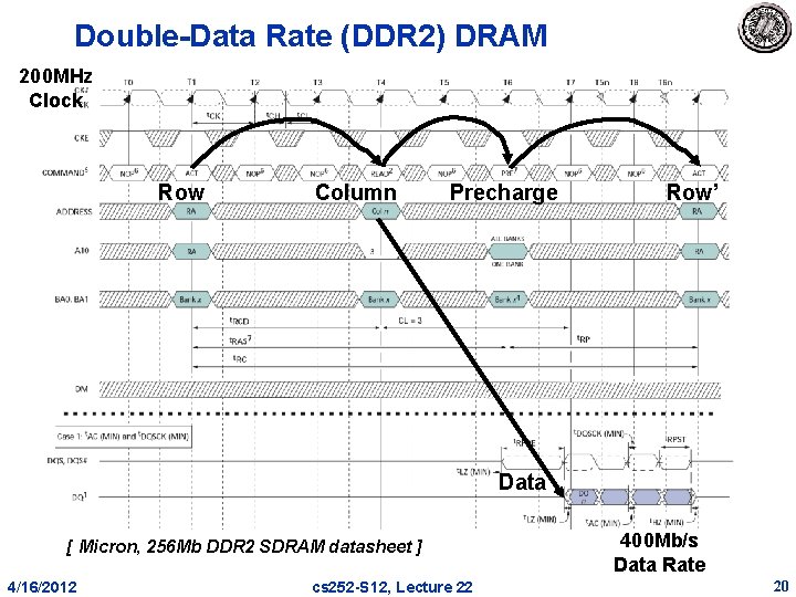
Quest for DRAM Performance 1. Fast Page mode – Add timing signals that allow repeated accesses to row buffer without another row access time – Such a buffer comes naturally, as each array will buffer 1024 to 2048 bits for each access 2. Synchronous DRAM (SDRAM) – Add a clock signal to DRAM interface, so that the repeated transfers would not bear overhead to synchronize with DRAM controller 3. Double Data Rate (DDR SDRAM) – Transfer data on both the rising edge and falling edge of the DRAM clock signal doubling the peak data rate – DDR 2 lowers power by dropping the voltage from 2. 5 to 1. 8 volts + offers higher clock rates: up to 400 MHz – DDR 3 drops to 1. 5 volts + higher clock rates: up to 800 MHz • 4/16/2012 Improved Bandwidth, not Latency cs 252 S 12, Lecture 22 16

Fast Memory Systems: DRAM specific • Multiple CAS accesses: several names (page mode) – Extended Data Out (EDO): 30% faster in page mode • Newer DRAMs to address gap; what will they cost, will they survive? – RAMBUS: startup company; reinvented DRAM interface » Each Chip a module vs. slice of memory » Short bus between CPU and chips » Does own refresh » Variable amount of data returned » 1 byte / 2 ns (500 MB/s per chip) – Synchronous DRAM: 2 banks on chip, a clock signal to DRAM, transfer synchronous to system clock (66 150 MHz) » DDR DRAM: Two transfers per clock (on rising and falling edge) – Intel claims FB-DIMM is the next big thing » Stands for “Fully Buffered Dual Inline RAM” » Same basic technology as DDR, but utilizes a serial “daisy chain” channel between different memory components. 4/16/2012 cs 252 S 12, Lecture 22 17

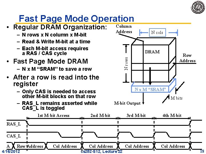
Fast Page Mode Operation • Regular DRAM Organization: – N rows x N column x M bit – Read & Write M bit at a time – Each M bit access requires a RAS / CAS cycle Column Address DRAM – N x M “SRAM” to save a row • After a row is read into the register – Only CAS is needed to access other M bit blocks on that row – RAS_L remains asserted while CAS_L is toggled Row Address N rows • Fast Page Mode DRAM 1 st M-bit Access N cols N x M “SRAM” M bits M-bit Output 2 nd M-bit 3 rd M-bit 4 th M-bit Col Address RAS_L CAS_L A Row Address 4/16/2012 Col Address cs 252 S 12, Lecture 22 18

SDRAM timing (Single Data Rate) CAS RAS (New Bank) x CAS Latency Precharge Burst READ • Micron 128 M bit dram (using 2 Meg 16 bit 4 bank ver) – Row (12 bits), bank (2 bits), column (9 bits) 4/16/2012 cs 252 S 12, Lecture 22 19

Double Data Rate (DDR 2) DRAM 200 MHz Clock Row Column Precharge Row’ Data [ Micron, 256 Mb DDR 2 SDRAM datasheet ] 4/16/2012 cs 252 S 12, Lecture 22 400 Mb/s Data Rate 20

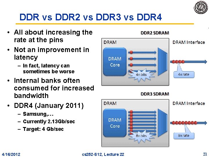
DDR vs DDR 2 vs DDR 3 vs DDR 4 • All about increasing the rate at the pins • Not an improvement in latency – In fact, latency can sometimes be worse • Internal banks often consumed for increased bandwidth • DDR 4 (January 2011) – Samsung, … – Currently 2. 13 Gb/sec – Target: 4 Gb/sec 4/16/2012 cs 252 S 12, Lecture 22 21

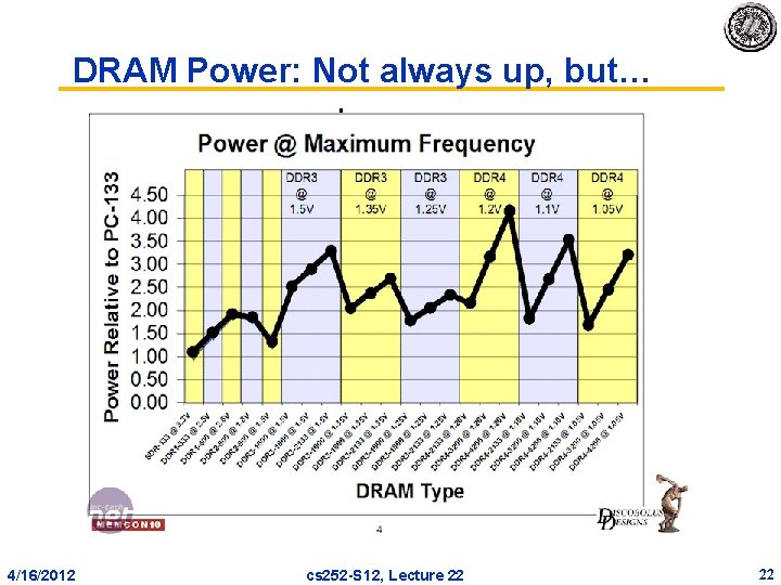
DRAM Power: Not always up, but… 4/16/2012 cs 252 S 12, Lecture 22 22

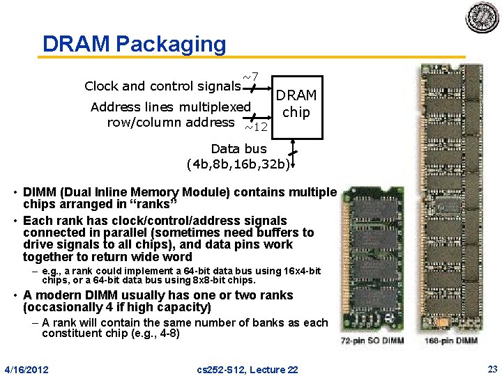
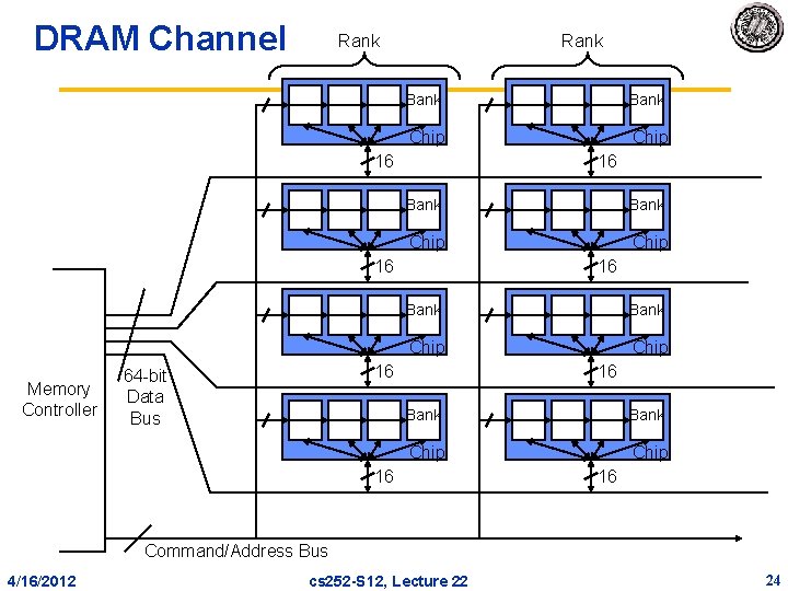
DRAM Packaging Clock and control signals ~7 Address lines multiplexed row/column address ~12 DRAM chip Data bus (4 b, 8 b, 16 b, 32 b) • DIMM (Dual Inline Memory Module) contains multiple chips arranged in “ranks” • Each rank has clock/control/address signals connected in parallel (sometimes need buffers to drive signals to all chips), and data pins work together to return wide word – e. g. , a rank could implement a 64 bit data bus using 16 x 4 bit chips, or a 64 bit data bus using 8 x 8 bit chips. • A modern DIMM usually has one or two ranks (occasionally 4 if high capacity) – A rank will contain the same number of banks as each constituent chip (e. g. , 4 8) 4/16/2012 cs 252 S 12, Lecture 22 23

DRAM Channel Rank Bank Chip 16 16 Bank Chip 16 Memory Controller 16 Bank Chip 16 64 -bit Data Bus 16 Bank Chip 16 16 Command/Address Bus 4/16/2012 cs 252 S 12, Lecture 22 24

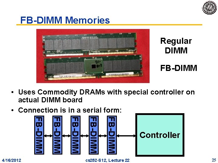
FB DIMM Memories Regular DIMM FB DIMM • Uses Commodity DRAMs with special controller on actual DIMM board • Connection is in a serial form: FB DIMM FB DIMM 4/16/2012 cs 252 S 12, Lecture 22 Controller 25

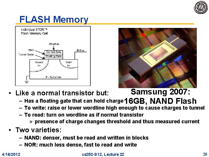
FLASH Memory Samsung 2007: – Has a floating gate that can hold charge 16 GB, NAND Flash • Like a normal transistor but: – To write: raise or lower wordline high enough to cause charges to tunnel – To read: turn on wordline as if normal transistor » presence of charge changes threshold and thus measured current • Two varieties: – NAND: denser, must be read and written in blocks – NOR: much less dense, fast to read and write 4/16/2012 cs 252 S 12, Lecture 22 26

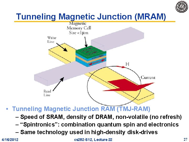
Tunneling Magnetic Junction (MRAM) • Tunneling Magnetic Junction RAM (TMJ RAM) – Speed of SRAM, density of DRAM, non volatile (no refresh) – “Spintronics”: combination quantum spin and electronics – Same technology used in high density disk drives 4/16/2012 cs 252 S 12, Lecture 22 27

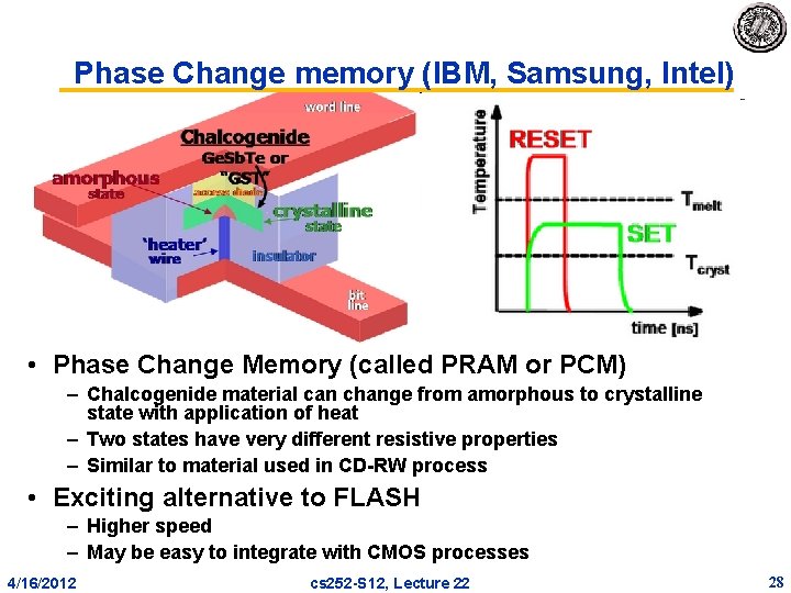
Phase Change memory (IBM, Samsung, Intel) • Phase Change Memory (called PRAM or PCM) – Chalcogenide material can change from amorphous to crystalline state with application of heat – Two states have very different resistive properties – Similar to material used in CD RW process • Exciting alternative to FLASH – Higher speed – May be easy to integrate with CMOS processes 4/16/2012 cs 252 S 12, Lecture 22 28

Error Correction Codes (ECC) • Memory systems generate errors (accidentally flipped bits) – DRAMs store very little charge per bit – “Soft” errors occur occasionally when cells are struck by alpha particles or other environmental upsets. – Less frequently, “hard” errors can occur when chips permanently fail. – Problem gets worse as memories get denser and larger • Where is “perfect” memory required? – servers, spacecraft/military computers, ebay, … • Memories are protected against failures with ECCs • Extra bits are added to each data word – used to detect and/or correct faults in the memory system – in general, each possible data word value is mapped to a unique “code word”. A fault changes a valid code word to an invalid one which can be detected. 4/16/2012 cs 252 S 12, Lecture 22 29

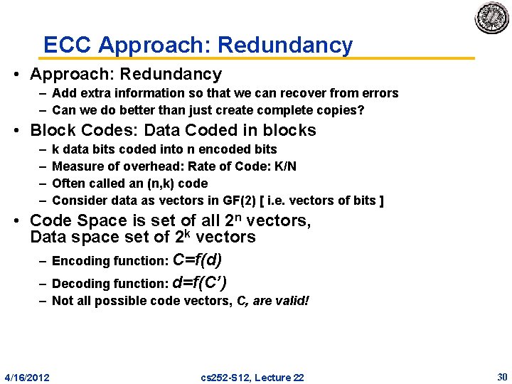
ECC Approach: Redundancy • Approach: Redundancy – Add extra information so that we can recover from errors – Can we do better than just create complete copies? • Block Codes: Data Coded in blocks – – k data bits coded into n encoded bits Measure of overhead: Rate of Code: K/N Often called an (n, k) code Consider data as vectors in GF(2) [ i. e. vectors of bits ] • Code Space is set of all 2 n vectors, Data space set of 2 k vectors – Encoding function: C=f(d) – Decoding function: d=f(C’) – Not all possible code vectors, C, are valid! 4/16/2012 cs 252 S 12, Lecture 22 30

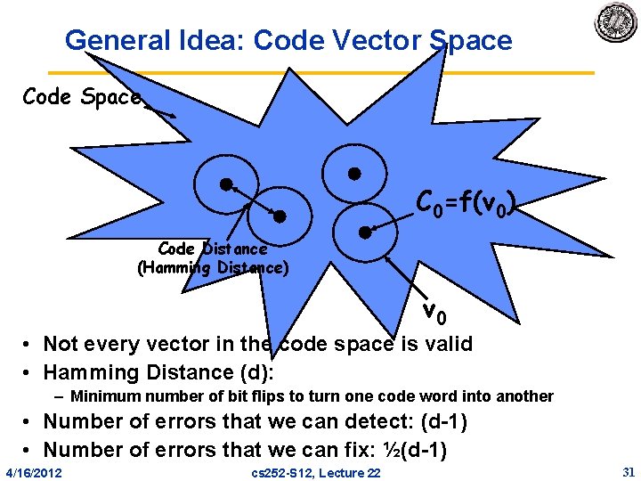
General Idea: Code Vector Space Code Space C 0=f(v 0) Code Distance (Hamming Distance) v 0 • Not every vector in the code space is valid • Hamming Distance (d): – Minimum number of bit flips to turn one code word into another • Number of errors that we can detect: (d 1) • Number of errors that we can fix: ½(d 1) 4/16/2012 cs 252 S 12, Lecture 22 31

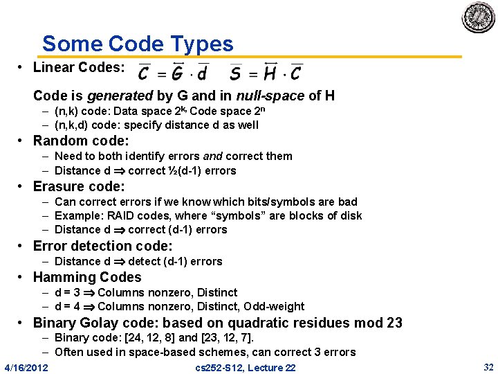
Some Code Types • Linear Codes: Code is generated by G and in null-space of H – (n, k) code: Data space 2 k, Code space 2 n – (n, k, d) code: specify distance d as well • Random code: – Need to both identify errors and correct them – Distance d correct ½(d 1) errors • Erasure code: – Can correct errors if we know which bits/symbols are bad – Example: RAID codes, where “symbols” are blocks of disk – Distance d correct (d 1) errors • Error detection code: – Distance d detect (d 1) errors • Hamming Codes – d = 3 Columns nonzero, Distinct – d = 4 Columns nonzero, Distinct, Odd weight • Binary Golay code: based on quadratic residues mod 23 – Binary code: [24, 12, 8] and [23, 12, 7]. – Often used in space based schemes, can correct 3 errors 4/16/2012 cs 252 S 12, Lecture 22 32

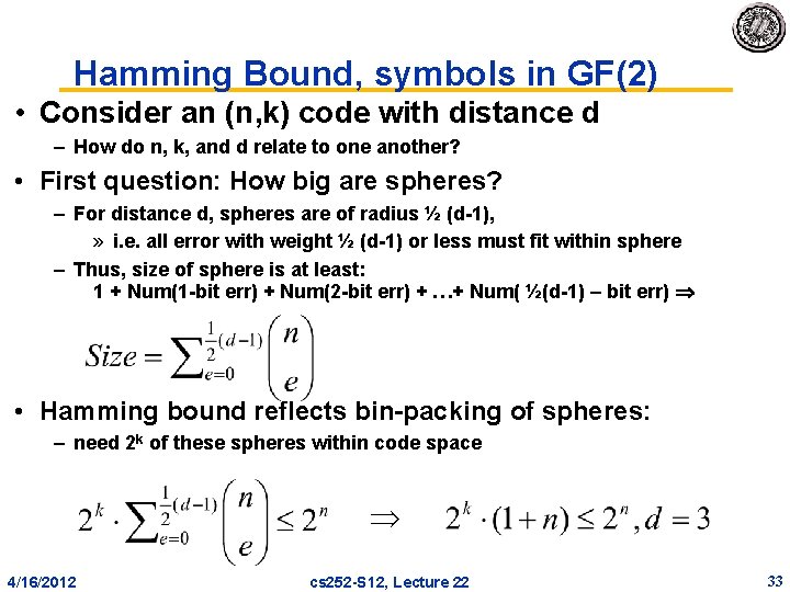
Hamming Bound, symbols in GF(2) • Consider an (n, k) code with distance d – How do n, k, and d relate to one another? • First question: How big are spheres? – For distance d, spheres are of radius ½ (d 1), » i. e. all error with weight ½ (d 1) or less must fit within sphere – Thus, size of sphere is at least: 1 + Num(1 bit err) + Num(2 bit err) + …+ Num( ½(d 1) – bit err) • Hamming bound reflects bin packing of spheres: – need 2 k of these spheres within code space 4/16/2012 cs 252 S 12, Lecture 22 33

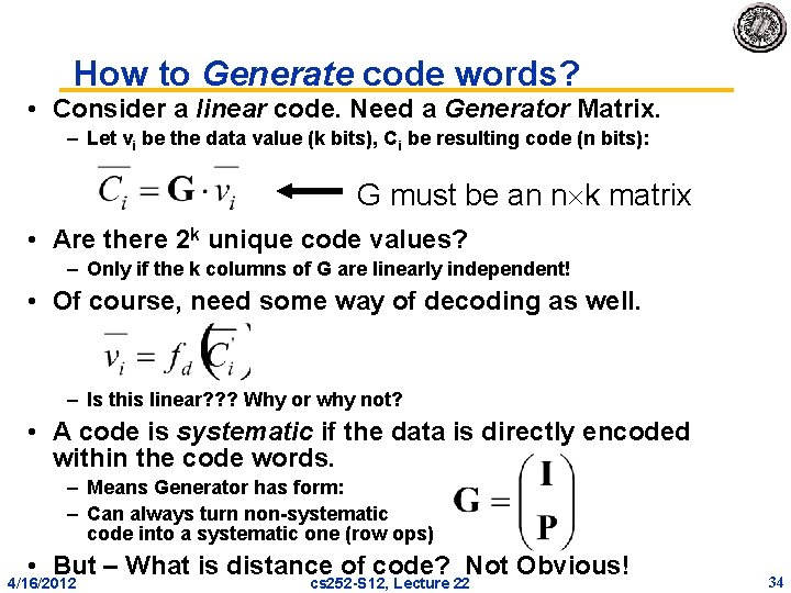
How to Generate code words? • Consider a linear code. Need a Generator Matrix. – Let vi be the data value (k bits), Ci be resulting code (n bits): G must be an n k matrix • Are there 2 k unique code values? – Only if the k columns of G are linearly independent! • Of course, need some way of decoding as well. – Is this linear? ? ? Why or why not? • A code is systematic if the data is directly encoded within the code words. – Means Generator has form: – Can always turn non systematic code into a systematic one (row ops) • But – What is distance of code? Not Obvious! 4/16/2012 cs 252 S 12, Lecture 22 34

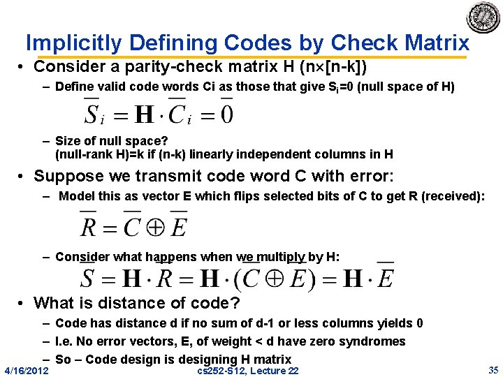
Implicitly Defining Codes by Check Matrix • Consider a parity check matrix H (n [n k]) – Define valid code words Ci as those that give Si=0 (null space of H) – Size of null space? (null rank H)=k if (n k) linearly independent columns in H • Suppose we transmit code word C with error: – Model this as vector E which flips selected bits of C to get R (received): – Consider what happens when we multiply by H: • What is distance of code? – Code has distance d if no sum of d 1 or less columns yields 0 – I. e. No error vectors, E, of weight < d have zero syndromes – So – Code design is designing H matrix 4/16/2012 cs 252 S 12, Lecture 22 35

How to relate G and H (Binary Codes) • Defining H makes it easy to understand distance of code, but hard to generate code (H defines code implicitly!) • However, let H be of following form: P is (n-k) k, I is (n-k) Result: H is (n-k) n • Then, G can be of following form (maximal code size): P is (n-k) k, I is k k Result: G is n k • Notice: G generates values in null space of H and has k independent columns so generates 2 k unique values: 4/16/2012 cs 252 S 12, Lecture 22 36

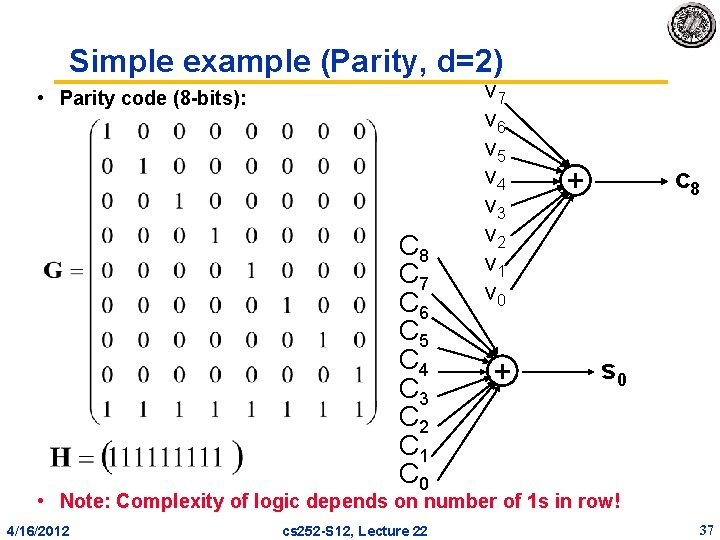
Simple example (Parity, d=2) • Parity code (8 bits): C 8 C 7 C 6 C 5 C 4 C 3 C 2 C 1 C 0 v 7 v 6 v 5 v 4 v 3 v 2 v 1 v 0 + c 8 + s 0 • Note: Complexity of logic depends on number of 1 s in row! 4/16/2012 cs 252 S 12, Lecture 22 37

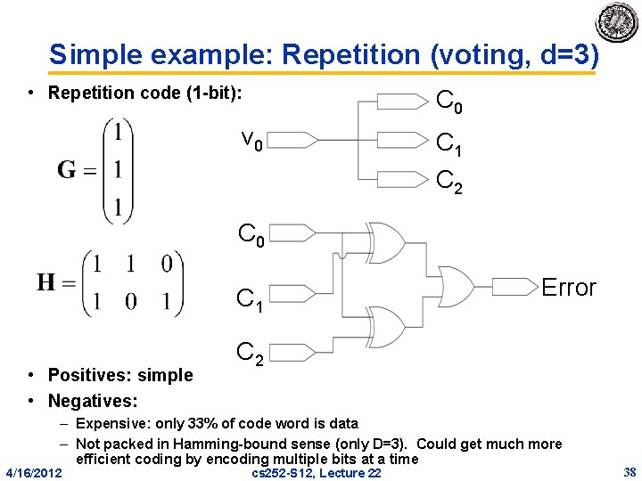
Simple example: Repetition (voting, d=3) • Repetition code (1 bit): C 0 v 0 C 1 C 2 C 0 C 1 • Positives: simple • Negatives: Error C 2 – Expensive: only 33% of code word is data – Not packed in Hamming bound sense (only D=3). Could get much more efficient coding by encoding multiple bits at a time 4/16/2012 cs 252 S 12, Lecture 22 38

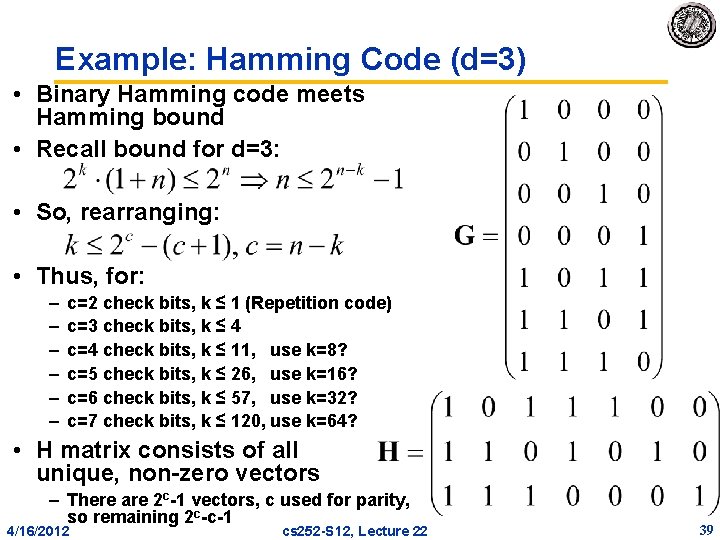
Example: Hamming Code (d=3) • Binary Hamming code meets Hamming bound • Recall bound for d=3: • So, rearranging: • Thus, for: – – – c=2 check bits, k ≤ 1 (Repetition code) c=3 check bits, k ≤ 4 c=4 check bits, k ≤ 11, use k=8? c=5 check bits, k ≤ 26, use k=16? c=6 check bits, k ≤ 57, use k=32? c=7 check bits, k ≤ 120, use k=64? • H matrix consists of all unique, non zero vectors – There are 2 c 1 vectors, c used for parity, so remaining 2 c c 1 4/16/2012 cs 252 S 12, Lecture 22 39

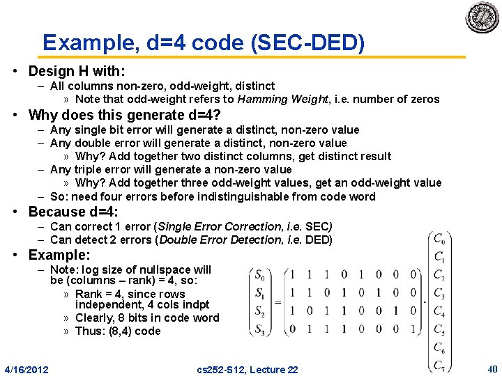
Example, d=4 code (SEC DED) • Design H with: – All columns non zero, odd weight, distinct » Note that odd weight refers to Hamming Weight, i. e. number of zeros • Why does this generate d=4? – Any single bit error will generate a distinct, non zero value – Any double error will generate a distinct, non zero value » Why? Add together two distinct columns, get distinct result – Any triple error will generate a non zero value » Why? Add together three odd weight values, get an odd weight value – So: need four errors before indistinguishable from code word • Because d=4: – Can correct 1 error (Single Error Correction, i. e. SEC) – Can detect 2 errors (Double Error Detection, i. e. DED) • Example: – Note: log size of nullspace will be (columns – rank) = 4, so: » Rank = 4, since rows independent, 4 cols indpt » Clearly, 8 bits in code word » Thus: (8, 4) code 4/16/2012 cs 252 S 12, Lecture 22 40

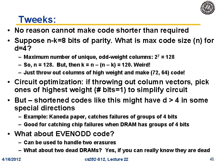
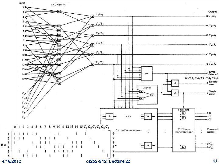
Tweeks: • No reason cannot make code shorter than required • Suppose n k=8 bits of parity. What is max code size (n) for d=4? – Maximum number of unique, odd weight columns: 27 = 128 – So, n = 128. But, then k = n – (n – k) = 120. Weird! – Just throw out columns of high weight and make (72, 64) code! • Circuit optimization: if throwing out column vectors, pick ones of highest weight (# bits=1) to simplify circuit • But – shortened codes like this might have d > 4 in some special directions – Example: Kaneda paper, catches failures of groups of 4 bits – Good for catching chip failures when DRAM has groups of 4 bits • What about EVENODD code? – Can be used to handle two erasures – What about two dead DRAMs? Yes, if you can really know they are dead 4/16/2012 cs 252 S 12, Lecture 22 41

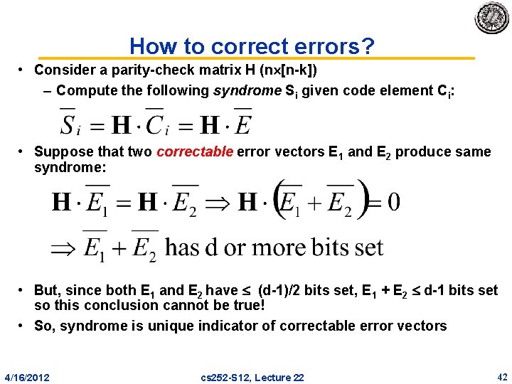
How to correct errors? • Consider a parity check matrix H (n [n k]) – Compute the following syndrome Si given code element Ci: • Suppose that two correctable error vectors E 1 and E 2 produce same syndrome: • But, since both E 1 and E 2 have (d 1)/2 bits set, E 1 + E 2 d 1 bits set so this conclusion cannot be true! • So, syndrome is unique indicator of correctable error vectors 4/16/2012 cs 252 S 12, Lecture 22 42

4/16/2012 cs 252 S 12, Lecture 22 43

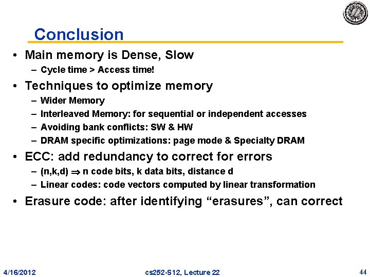
Conclusion • Main memory is Dense, Slow – Cycle time > Access time! • Techniques to optimize memory – – Wider Memory Interleaved Memory: for sequential or independent accesses Avoiding bank conflicts: SW & HW DRAM specific optimizations: page mode & Specialty DRAM • ECC: add redundancy to correct for errors – (n, k, d) n code bits, k data bits, distance d – Linear codes: code vectors computed by linear transformation • Erasure code: after identifying “erasures”, can correct 4/16/2012 cs 252 S 12, Lecture 22 44