Course Outline Traditional Static Program Analysis Theory Compiler

Course Outline • Traditional Static Program Analysis – Theory • Compiler Optimizations; Control Flow Graphs • Data-flow Analysis – today’s class – Classic analyses and applications • Software Testing • Dynamic Program Analysis

Announcements • Next time: Homework 1 will be posted at: – www. cs. rpi. edu/~milanova/csci 6961/ – Due next Thursday, Feb 17 th – There will be 3 homework assignments

Outline • The four classical data-flow problems, continue – – Reaching definitions Live variables Available expressions Very busy expressions • Data-flow frameworks • Reading: Compilers: Principles, Techniques and Tools, by Aho, Lam, Sethi and Ullman, Chapter 9. 2 and 9. 3

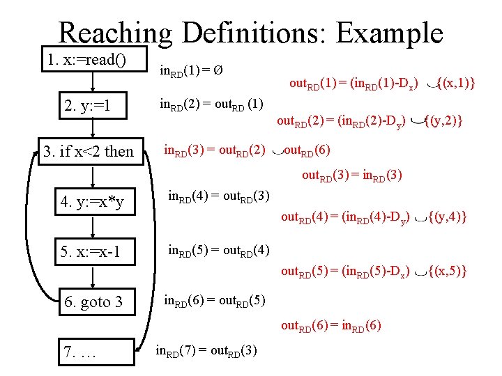
Reaching Definitions: Example 1. x: =read() in. RD(1) = Ø 2. y: =1 in. RD(2) = out. RD (1) 3. if x<2 then in. RD(3) = out. RD(2) out. RD(1) = (in. RD(1)-Dx) out. RD(2) = (in. RD(2)-Dy) {(x, 1)} {(y, 2)} out. RD(6) out. RD(3) = in. RD(3) 4. y: =x*y in. RD(4) = out. RD(3) 5. x: =x-1 in. RD(5) = out. RD(4) 6. goto 3 out. RD(4) = (in. RD(4)-Dy) {(y, 4)} out. RD(5) = (in. RD(5)-Dx) {(x, 5)} in. RD(6) = out. RD(5) out. RD(6) = in. RD(6) 7. … in. RD(7) = out. RD(3)

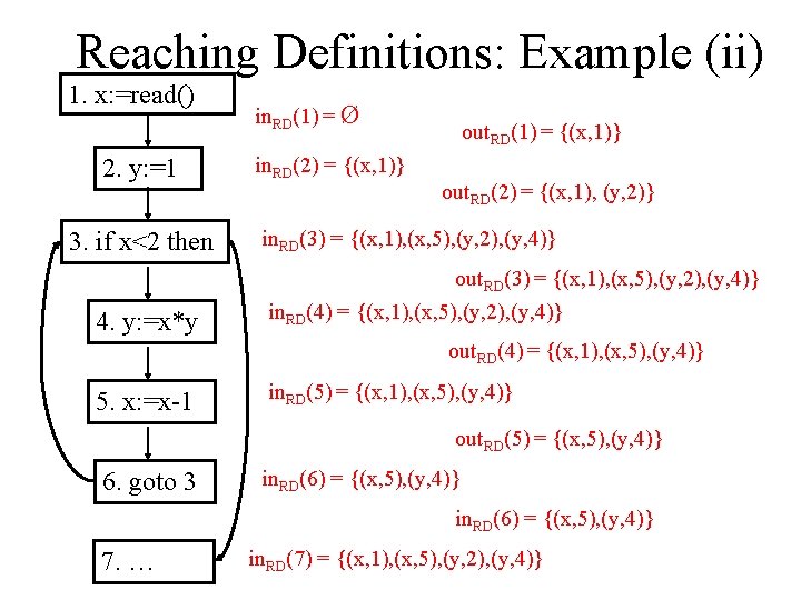
Reaching Definitions: Example (ii) 1. x: =read() 2. y: =1 3. if x<2 then in. RD(1) = Ø in. RD(2) = {(x, 1)} out. RD(1) = {(x, 1)} out. RD(2) = {(x, 1), (y, 2)} in. RD(3) = {(x, 1), (x, 5), (y, 2), (y, 4)} out. RD(3) = {(x, 1), (x, 5), (y, 2), (y, 4)} 4. y: =x*y in. RD(4) = {(x, 1), (x, 5), (y, 2), (y, 4)} out. RD(4) = {(x, 1), (x, 5), (y, 4)} 5. x: =x-1 in. RD(5) = {(x, 1), (x, 5), (y, 4)} out. RD(5) = {(x, 5), (y, 4)} 6. goto 3 in. RD(6) = {(x, 5), (y, 4)} 7. … in. RD(7) = {(x, 1), (x, 5), (y, 2), (y, 4)}

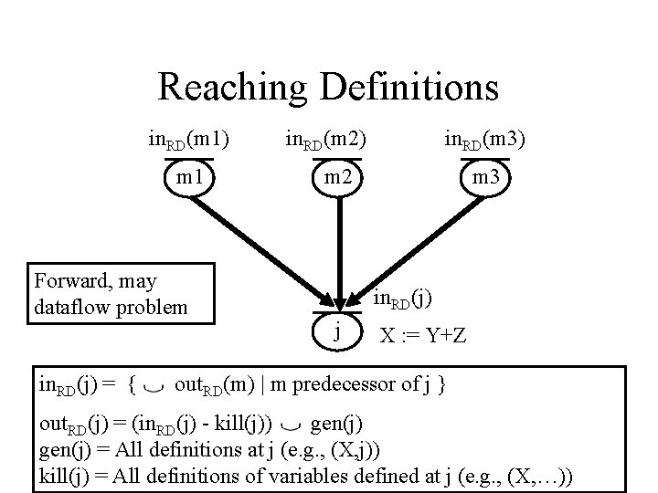
Reaching Definitions in. RD(m 1) m 1 Forward, may dataflow problem in. RD(j) = { in. RD(m 2) in. RD(m 3) m 2 m 3 in. RD(j) j X : = Y+Z out. RD(m) | m predecessor of j } out. RD(j) = (in. RD(j) - kill(j)) gen(j) = All definitions at j (e. g. , (X, j)) kill(j) = All definitions of variables defined at j (e. g. , (X, …))

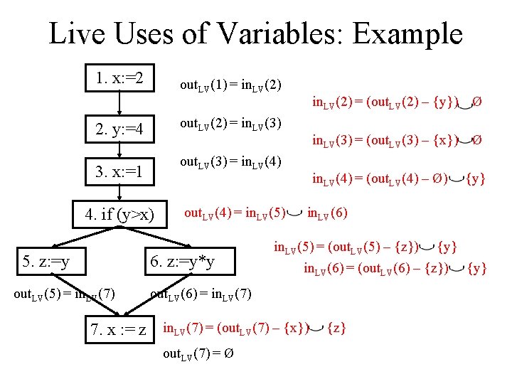
Live Uses of Variables: Example 1. x: =2 out. LV(1) = in. LV(2) out. LV(2) = in. LV(3) 2. y: =4 out. LV(3) = in. LV(4) 3. x: =1 4. if (y>x) 5. z: =y out. LV(4) = in. LV(5) 6. z: =y*y out. LV(5) = in. LV(7) in. LV(2) = (out. LV(2) – {y}) Ø in. LV(3) = (out. LV(3) – {x}) Ø in. LV(4) = (out. LV(4) – Ø) in. LV(6) in. LV(5) = (out. LV(5) – {z}) {y} in. LV(6) = (out. LV(6) – {z}) {y} out. LV(6) = in. LV(7) 7. x : = z in. LV(7) = (out. LV(7) – {x}) out. LV(7) = Ø {y} {z}

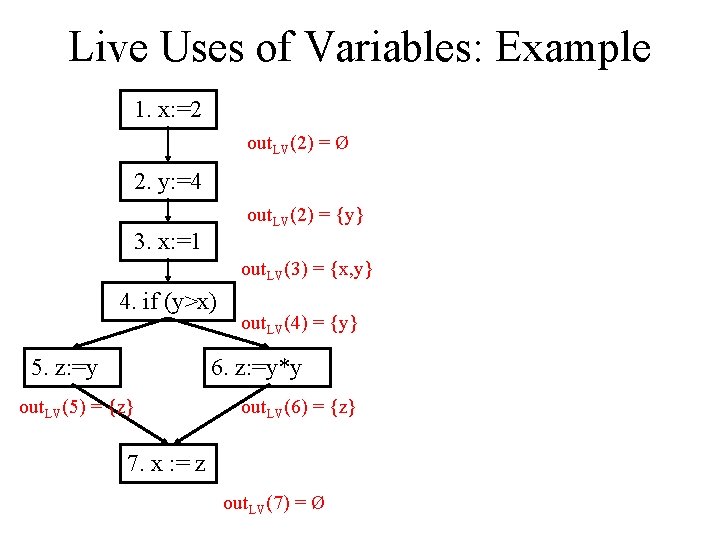
Live Uses of Variables: Example 1. x: =2 out. LV(2) = Ø 2. y: =4 out. LV(2) = {y} 3. x: =1 out. LV(3) = {x, y} 4. if (y>x) 5. z: =y out. LV(4) = {y} 6. z: =y*y out. LV(5) = {z} out. LV(6) = {z} 7. x : = z out. LV(7) = Ø

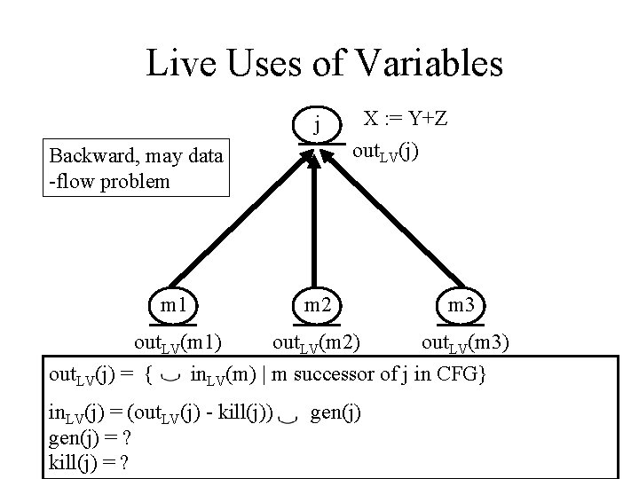
Live Uses of Variables X : = Y+Z j out. LV(j) Backward, may data -flow problem m 1 m 2 m 3 out. LV(m 1) out. LV(m 2) out. LV(m 3) out. LV(j) = { in. LV(m) | m successor of j in CFG} in. LV(j) = (out. LV(j) - kill(j)) gen(j) = ? kill(j) = ? gen(j)

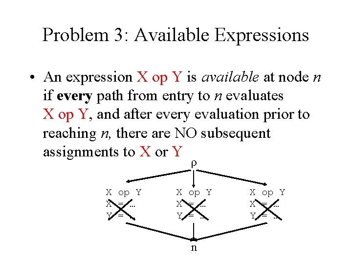
Problem 3: Available Expressions • An expression X op Y is available at node n if every path from entry to n evaluates X op Y, and after every evaluation prior to reaching n, there are NO subsequent assignments to X or Y ρ X op Y X = … Y = … n X op Y X = … Y = …

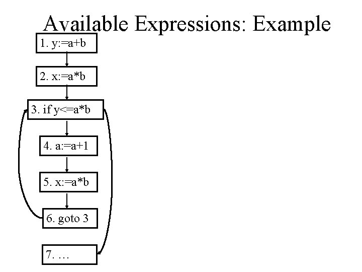
Available Expressions: Example 1. y: =a+b 2. x: =a*b 3. if y<=a*b 4. a: =a+1 5. x: =a*b 6. goto 3 7. …

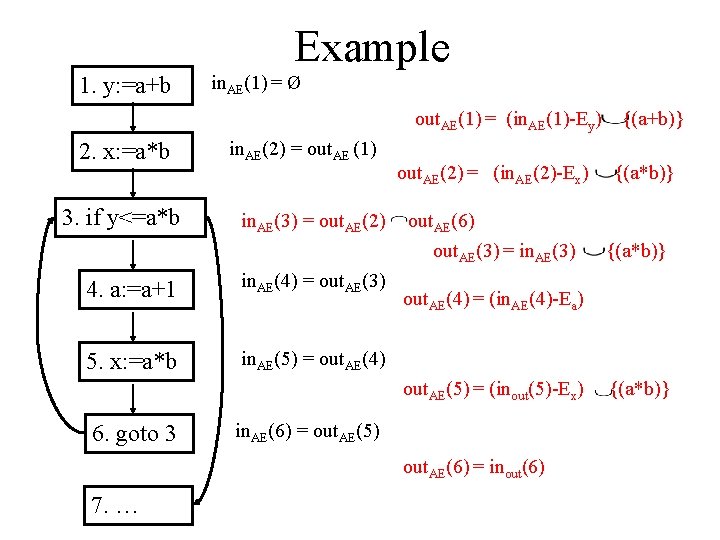
Example 1. y: =a+b in. AE(1) = Ø out. AE(1) = (in. AE(1)-Ey) 2. x: =a*b 3. if y<=a*b in. AE(2) = out. AE (1) in. AE(3) = out. AE(2) 4. a: =a+1 in. AE(4) = out. AE(3) 5. x: =a*b in. AE(5) = out. AE(4) out. AE(2) = (in. AE(2)-Ex) out. AE(6) out. AE(3) = in. AE(3) in. AE(6) = out. AE(5) out. AE(6) = inout(6) 7. … {(a*b)} out. AE(4) = (in. AE(4)-Ea) out. AE(5) = (inout(5)-Ex) 6. goto 3 {(a+b)} {(a*b)}

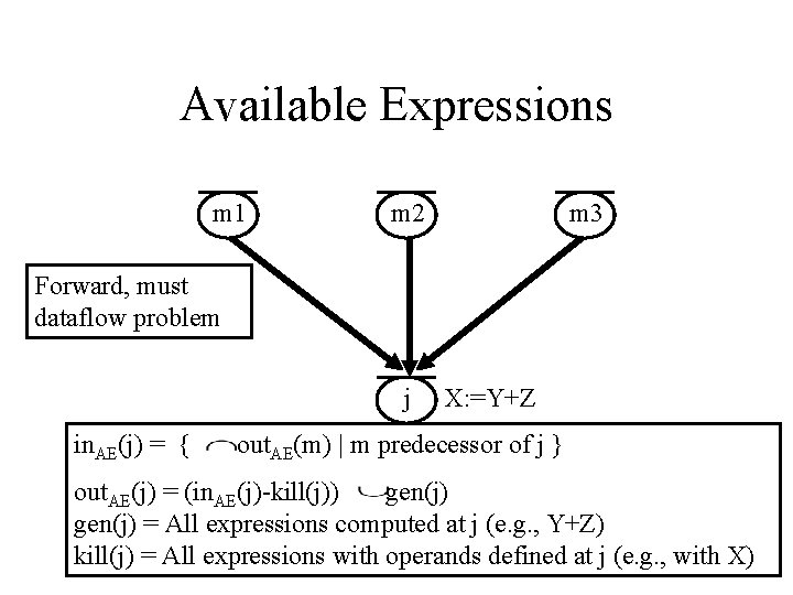
Available Expressions m 1 m 2 m 3 Forward, must dataflow problem j in. AE(j) = { X: =Y+Z out. AE(m) | m predecessor of j } out. AE(j) = (in. AE(j)-kill(j)) gen(j) = All expressions computed at j (e. g. , Y+Z) kill(j) = All expressions with operands defined at j (e. g. , with X)

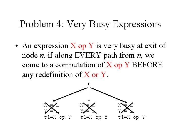
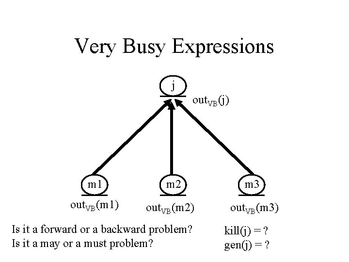
Problem 4: Very Busy Expressions • An expression X op Y is very busy at exit of node n, if along EVERY path from n, we come to a computation of X op Y BEFORE any redefinition of X or Y. n X = … Y = … t 1=X op Y

Very Busy Expressions j out. VB(j) m 1 out. VB(m 1) m 2 out. VB(m 2) Is it a forward or a backward problem? Is it a may or a must problem? m 3 out. VB(m 3) kill(j) = ? gen(j) = ?

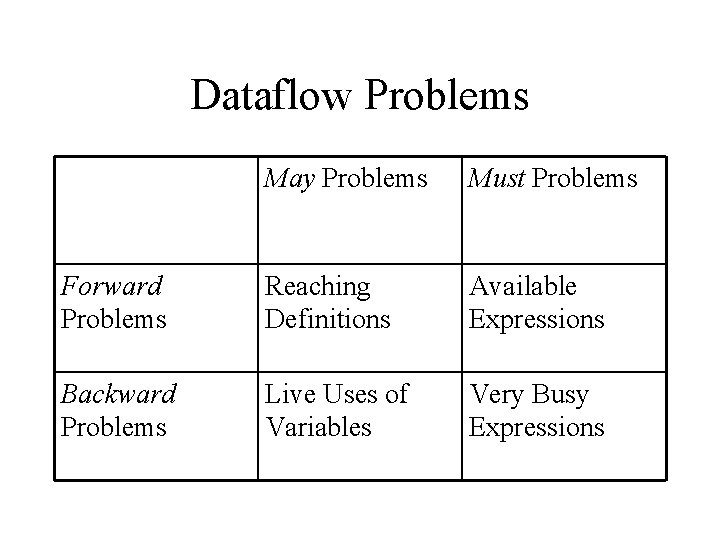
Dataflow Problems May Problems Must Problems Forward Problems Reaching Definitions Available Expressions Backward Problems Live Uses of Variables Very Busy Expressions

Similarities • There is a finite set U of dataflow facts: – Reaching Definitions: the set of all definitions in program – Live Uses of Variables: the set of all variables – Available Expressions and Very Busy Expressions: the set of all expressions in program • The solution at a node i (i. e. , in(i), out(i)) is a subset of U (e. g. , for each definition it either reaches program point i or does not).

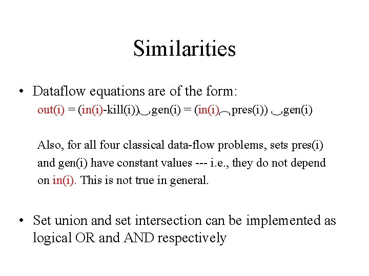
Similarities • Dataflow equations are of the form: out(i) = (in(i)-kill(i)) gen(i) = (in(i) pres(i)) gen(i) Also, for all four classical data-flow problems, sets pres(i) and gen(i) have constant values --- i. e. , they do not depend on in(i). This is not true in general. • Set union and set intersection can be implemented as logical OR and AND respectively

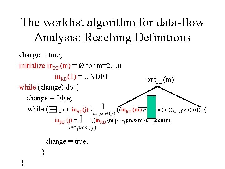
The worklist algorithm for data-flow Analysis: Reaching Definitions change = true; initialize in. RD(m) = Ø for m=2…n in. RD(1) = UNDEF out. RD(m) while (change) do { change = false; while ( j s. t. in. RD(j) ≠ ((in. RD (m) pres(m)) gen(m)) { in. RD (j) = change = true; } } ((in. RD (m) pres(m)) gen(m)

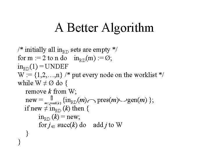
A Better Algorithm /* initially all in. RD sets are empty */ for m : = 2 to n do in. RD(m) : = Ø; in. RD(1) = UNDEF W : = {1, 2, …, n} /* put every node on the worklist */ while W ≠ Ø do { remove k from W; new = {in. RD(m) pres(m) gen(m) }; if new ≠ in. RD (k) then { in. RD (k) = new; for j succ(k) do add j to W } }

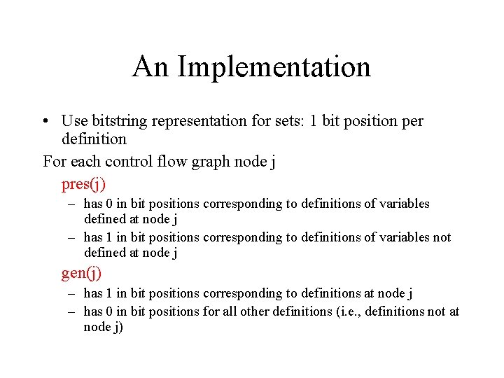
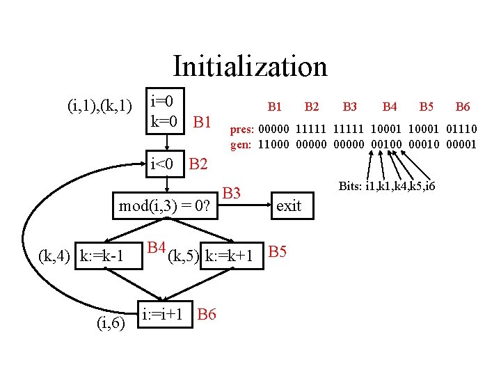
An Implementation • Use bitstring representation for sets: 1 bit position per definition For each control flow graph node j pres(j) – has 0 in bit positions corresponding to definitions of variables defined at node j – has 1 in bit positions corresponding to definitions of variables not defined at node j gen(j) – has 1 in bit positions corresponding to definitions at node j – has 0 in bit positions for all other definitions (i. e. , definitions not at node j)

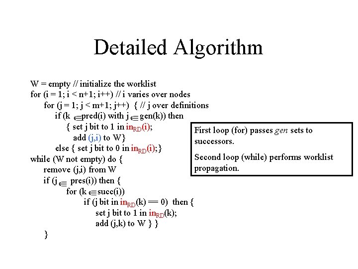
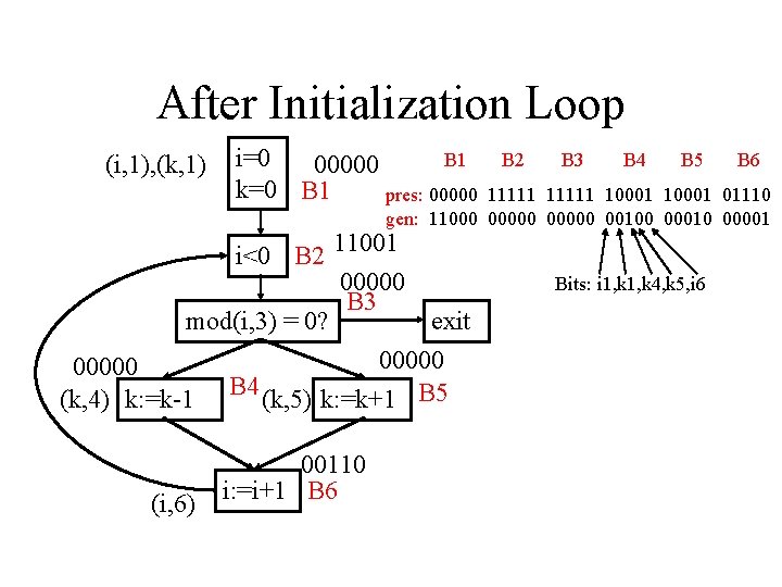
Detailed Algorithm W = empty // initialize the worklist for (i = 1; i < n+1; i++) // i varies over nodes for (j = 1; j < m+1; j++) { // j over definitions if (k pred(i) with j gen(k)) then { set j bit to 1 in in. RD(i); First loop (for) passes gen sets to add (j, i) to W} successors. else { set j bit to 0 in in. RD(i); } Second loop (while) performs worklist while (W not empty) do { propagation. remove (j, i) from W if (j pres(i)) then { for (k succ(i)) if (j bit in in. RD(k) == 0) then { set j bit to 1 in in. RD(k); add (j, k) to W } } }

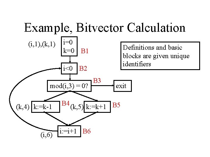
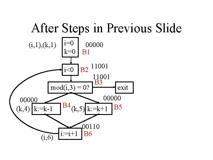
Example, Bitvector Calculation (i, 1), (k, 1) i=0 k=0 B 1 Definitions and basic blocks are given unique identifiers i<0 B 2 mod(i, 3) = 0? (k, 4) k: =k-1 (i, 6) B 3 exit B 4 (k, 5) k: =k+1 B 5 i: =i+1 B 6

Initialization (i, 1), (k, 1) i=0 k=0 B 1 B 2 B 3 B 4 B 5 pres: 00000 11111 10001 01110 gen: 11000 00000 00100 00010 00001 i<0 B 2 mod(i, 3) = 0? (k, 4) k: =k-1 (i, 6) B 3 Bits: i 1, k 4, k 5, i 6 exit B 4 (k, 5) k: =k+1 B 5 i: =i+1 B 6

After Initialization Loop (i, 1), (k, 1) i=0 B 1 00000 k=0 B 1 pres: 00000 B 2 B 3 B 4 B 5 B 6 11111 10001 01110 gen: 11000 00000 00100 00010 00001 i<0 B 2 11001 00000 B 3 mod(i, 3) = 0? exit 00000 (k, 4) k: =k-1 B 4 (k, 5) k: =k+1 B 5 (i, 6) 00110 i: =i+1 B 6 Bits: i 1, k 4, k 5, i 6

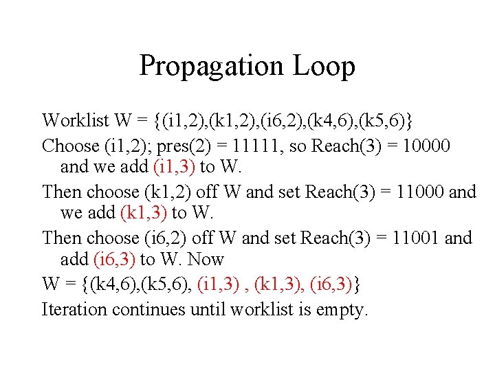
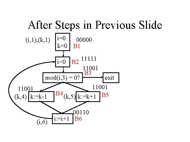
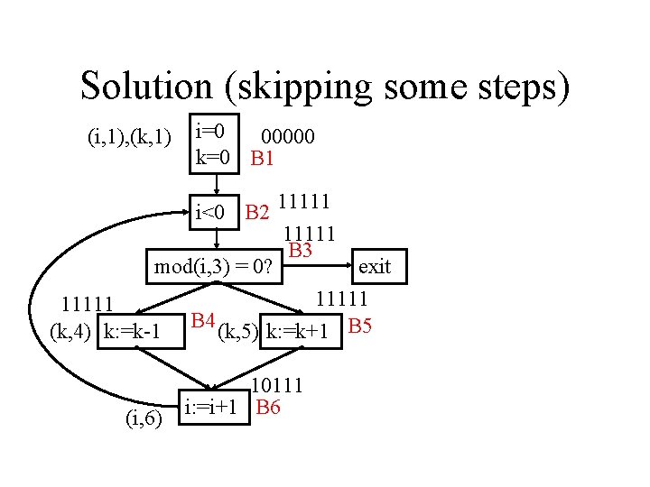
Propagation Loop Worklist W = {(i 1, 2), (k 1, 2), (i 6, 2), (k 4, 6), (k 5, 6)} Choose (i 1, 2); pres(2) = 11111, so Reach(3) = 10000 and we add (i 1, 3) to W. Then choose (k 1, 2) off W and set Reach(3) = 11000 and we add (k 1, 3) to W. Then choose (i 6, 2) off W and set Reach(3) = 11001 and add (i 6, 3) to W. Now W = {(k 4, 6), (k 5, 6), (i 1, 3) , (k 1, 3), (i 6, 3)} Iteration continues until worklist is empty.

After Steps in Previous Slide (i, 1), (k, 1) i=0 00000 k=0 B 1 i<0 B 2 11001 B 3 mod(i, 3) = 0? exit 00000 (k, 4) k: =k-1 B 4 (k, 5) k: =k+1 B 5 (i, 6) 00110 i: =i+1 B 6

After Steps in Previous Slide (i, 1), (k, 1) i=0 00000 k=0 B 1 i<0 B 2 11111 11001 B 3 mod(i, 3) = 0? exit 00000 (k, 4) k: =k-1 B 4 (k, 5) k: =k+1 B 5 (i, 6) 00110 i: =i+1 B 6

After Steps in Previous Slide (i, 1), (k, 1) i=0 00000 k=0 B 1 i<0 B 2 11111 11001 B 3 mod(i, 3) = 0? exit 11001 (k, 4) k: =k-1 B 4 (k, 5) k: =k+1 B 5 (i, 6) 00110 i: =i+1 B 6

Solution (skipping some steps) (i, 1), (k, 1) i=0 00000 k=0 B 1 i<0 B 2 11111 B 3 mod(i, 3) = 0? exit 11111 (k, 4) k: =k-1 B 4 (k, 5) k: =k+1 B 5 (i, 6) 10111 i: =i+1 B 6

Dataflow Frameworks • Lattice theoretic foundations – Partial ordering – Meet, Join, Lattice, and Chain • Monotone frameworks • The “Maximal Fixed Point” (MFP) solution • The “Meet Over all Paths” (MOP) solution

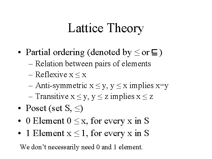
Lattice Theory • Partial ordering (denoted by ≤ or ) – Relation between pairs of elements – Reflexive x ≤ x – Anti-symmetric x ≤ y, y ≤ x implies x=y – Transitive x ≤ y, y ≤ z implies x ≤ z • Poset (set S, ≤) • 0 Element 0 ≤ x, for every x in S • 1 Element x ≤ 1, for every x in S We don’t necessarily need 0 and 1 element.

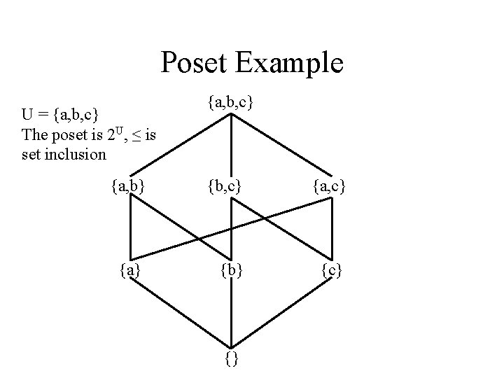
Poset Example U = {a, b, c} The poset is 2 U, ≤ is set inclusion {a, b, c} {a, b} {b, c} {a} {b} {c} {}

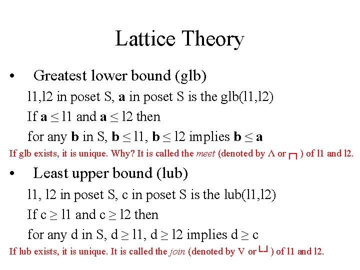
Lattice Theory • Greatest lower bound (glb) l 1, l 2 in poset S, a in poset S is the glb(l 1, l 2) If a ≤ l 1 and a ≤ l 2 then for any b in S, b ≤ l 1, b ≤ l 2 implies b ≤ a If glb exists, it is unique. Why? It is called the meet (denoted by Λ or┌┐) of l 1 and l 2. • Least upper bound (lub) l 1, l 2 in poset S, c in poset S is the lub(l 1, l 2) If c ≥ l 1 and c ≥ l 2 then for any d in S, d ≥ l 1, d ≥ l 2 implies d ≥ c If lub exists, it is unique. It is called the join (denoted by V or└┘) of l 1 and l 2.

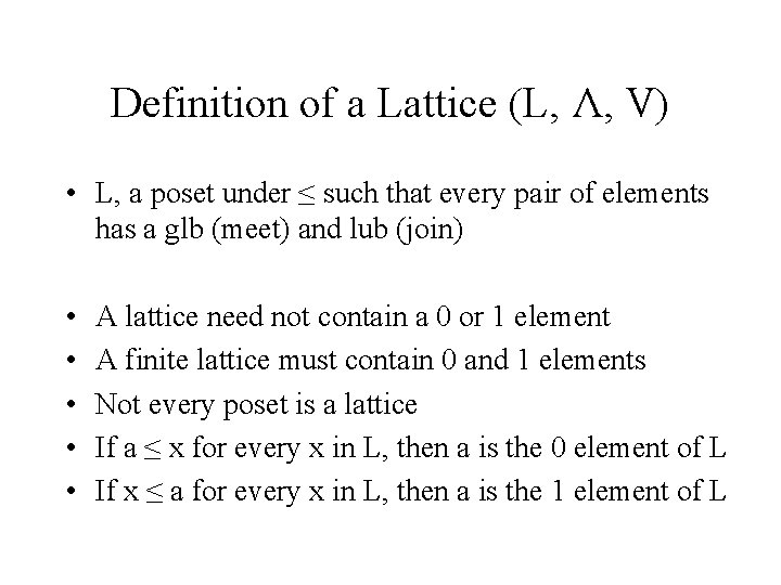
Definition of a Lattice (L, Λ, V) • L, a poset under ≤ such that every pair of elements has a glb (meet) and lub (join) • • • A lattice need not contain a 0 or 1 element A finite lattice must contain 0 and 1 elements Not every poset is a lattice If a ≤ x for every x in L, then a is the 0 element of L If x ≤ a for every x in L, then a is the 1 element of L

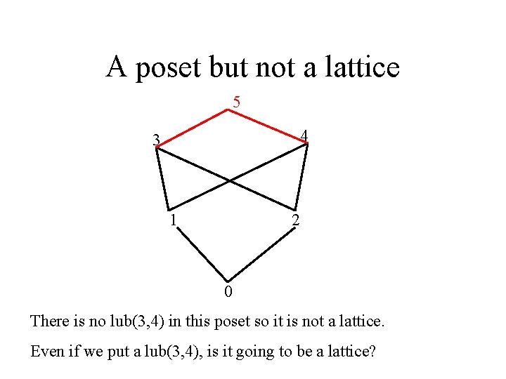
A poset but not a lattice 5 4 3 1 2 0 There is no lub(3, 4) in this poset so it is not a lattice. Even if we put a lub(3, 4), is it going to be a lattice?

Examples of Lattices • H = (2 U, ∩, U) where U is a finite set – glb(s 1, s 2) is (s 1Λs 2) which is s 1∩s 2 – lub(s 1, s 2) is (s 1 Vs 2) which is s 1 Us 2 • J = (N 1, gcd, lcm) – Partial order is integer divide on N 1 – lub(n 1, n 2) is (n 1 Vn 2) which is lcm(n 1, n 2) – glb(n 1, n 2) is (n 1Λn 2) which is gcd(n 1, n 2)

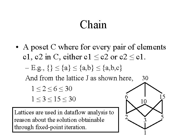
Chain • A poset C where for every pair of elements c 1, c 2 in C, either c 1 ≤ c 2 or c 2 ≤ c 1. – E. g. , {} ≤ {a, b} ≤ {a, b, c} And from the lattice J as shown here, 30 1 ≤ 2 ≤ 6 ≤ 30 6 1 ≤ 3 ≤ 15 ≤ 30 10 Lattices are used in dataflow analysis to reason about the solution obtainable through fixed-point iteration. 2 3 1 15 5