Course Outline Traditional Static Program Analysis Theory Compiler

Course Outline • Traditional Static Program Analysis – Theory • Compiler Optimizations; Control Flow Graphs • Data-flow Analysis – today’s class – Classic analyses and applications • Software Testing • Dynamic Program Analysis

Outline • The four classical data-flow problems – – Reaching definitions Live variables Available expressions Very busy expressions • Data-flow frameworks • Reading: Compilers: Principles, Techniques and Tools, by Aho, Lam, Sethi and Ullman, Chapter 9. 2��

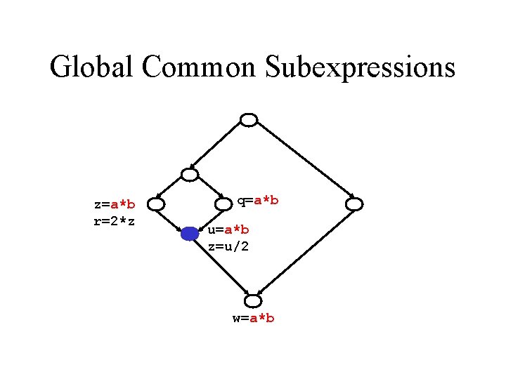
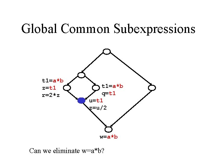
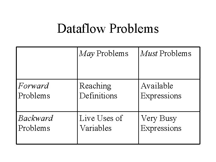
Four Classical Data-flow Problems • • • Reaching definitions (Reach) Live uses of variables (Live) Available expressions (Avail) Very busy expressions (Very. B) Def-use chains built from Reach, and the dual Use -def chains, built from Live, play role in many optimizations • Avail enables global common subexpression elimination • Very. B is used for conservative code motion

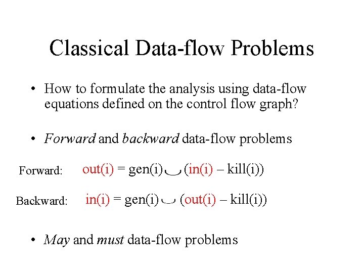
Classical Data-flow Problems • How to formulate the analysis using data-flow equations defined on the control flow graph? • Forward and backward data-flow problems Forward: out(i) = gen(i) (in(i) – kill(i)) Backward: in(i) = gen(i) (out(i) – kill(i)) • May and must data-flow problems

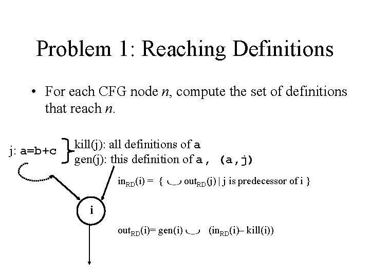
Problem 1: Reaching Definitions • For each CFG node n, compute the set of definitions that reach n. j: a=b+c kill(j): all definitions of a gen(j): this definition of a, (a, j) in. RD(i) = { out. RD(j) | j is predecessor of i } i out. RD(i)= gen(i) (in. RD(i)– kill(i))

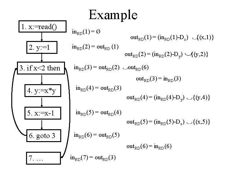
Example 1. x: =read() in. RD(1) = Ø 2. y: =1 in. RD(2) = out. RD (1) 3. if x<2 then in. RD(3) = out. RD(2) out. RD(1) = (in. RD(1)-Dx) out. RD(2) = (in. RD(2)-Dy) {(x, 1)} {(y, 2)} out. RD(6) out. RD(3) = in. RD(3) 4. y: =x*y in. RD(4) = out. RD(3) 5. x: =x-1 in. RD(5) = out. RD(4) 6. goto 3 out. RD(4) = (in. RD(4)-Dy) {(y, 4)} out. RD(5) = (in. RD(5)-Dx) {(x, 5)} in. RD(6) = out. RD(5) out. RD(6) = in. RD(6) 7. … in. RD(7) = out. RD(3)

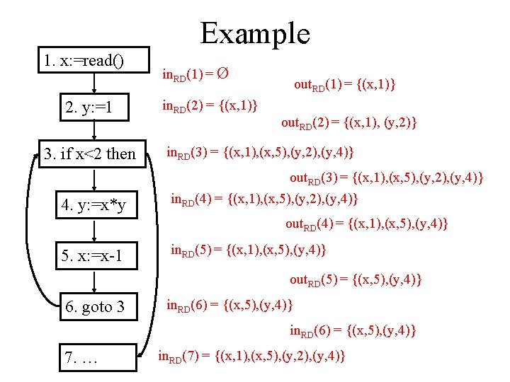
Example 1. x: =read() 2. y: =1 3. if x<2 then in. RD(1) = Ø in. RD(2) = {(x, 1)} out. RD(1) = {(x, 1)} out. RD(2) = {(x, 1), (y, 2)} in. RD(3) = {(x, 1), (x, 5), (y, 2), (y, 4)} out. RD(3) = {(x, 1), (x, 5), (y, 2), (y, 4)} 4. y: =x*y in. RD(4) = {(x, 1), (x, 5), (y, 2), (y, 4)} out. RD(4) = {(x, 1), (x, 5), (y, 4)} 5. x: =x-1 in. RD(5) = {(x, 1), (x, 5), (y, 4)} out. RD(5) = {(x, 5), (y, 4)} 6. goto 3 in. RD(6) = {(x, 5), (y, 4)} 7. … in. RD(7) = {(x, 1), (x, 5), (y, 2), (y, 4)}

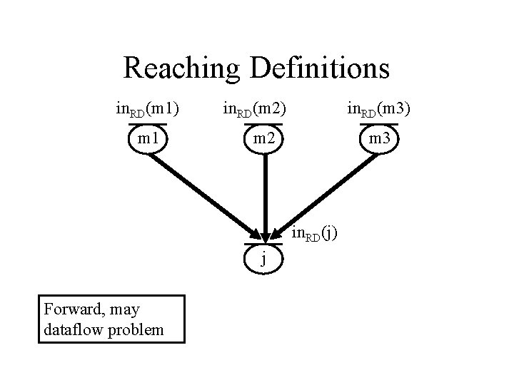
Reaching Definitions in. RD(m 1) m 1 in. RD(m 2) in. RD(m 3) m 2 m 3 in. RD(j) j Forward, may dataflow problem

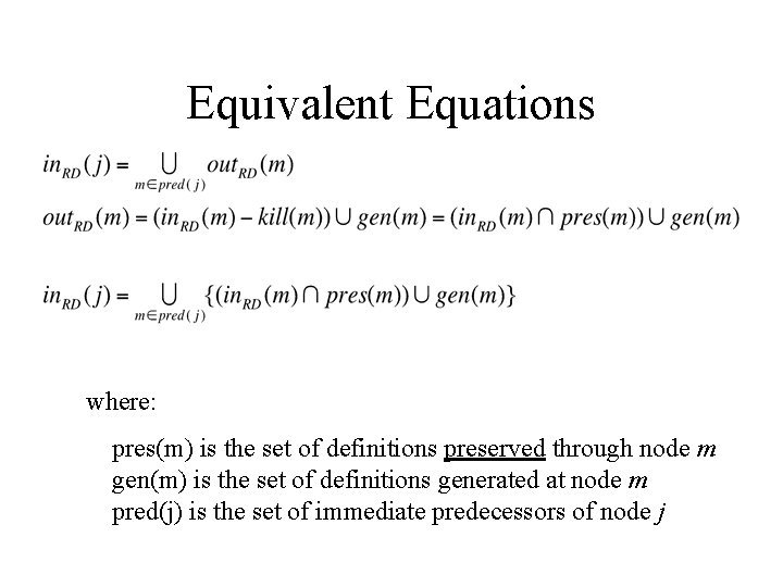
Equivalent Equations where: pres(m) is the set of definitions preserved through node m gen(m) is the set of definitions generated at node m pred(j) is the set of immediate predecessors of node j

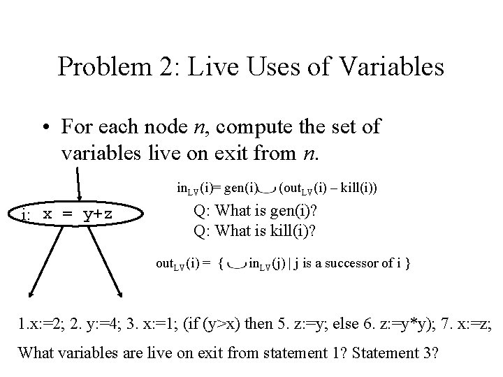
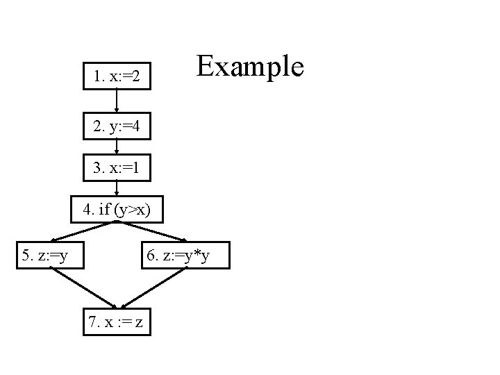
Problem 2: Live Uses of Variables • For each node n, compute the set of variables live on exit from n. in. LV(i)= gen(i) i: x = y+z (out. LV(i) – kill(i)) Q: What is gen(i)? Q: What is kill(i)? out. LV(i) = { in. LV(j) | j is a successor of i } 1. x: =2; 2. y: =4; 3. x: =1; (if (y>x) then 5. z: =y; else 6. z: =y*y); 7. x: =z; What variables are live on exit from statement 1? Statement 3?

Example 1. x: =2 2. y: =4 3. x: =1 4. if (y>x) 5. z: =y 6. z: =y*y 7. x : = z

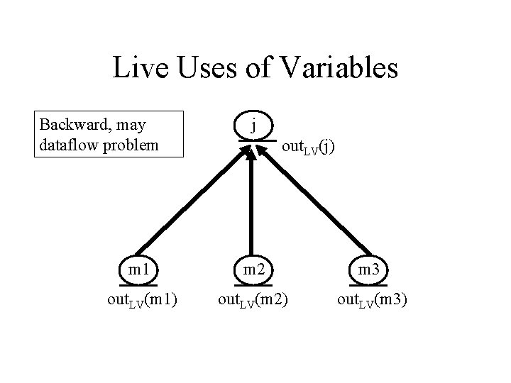
Live Uses of Variables Backward, may dataflow problem j out. LV(j) m 1 m 2 m 3 out. LV(m 1) out. LV(m 2) out. LV(m 3)

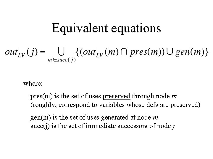
Equivalent equations where: pres(m) is the set of uses preserved through node m (roughly, correspond to variables whose defs are preserved) gen(m) is the set of uses generated at node m succ(j) is the set of immediate successors of node j

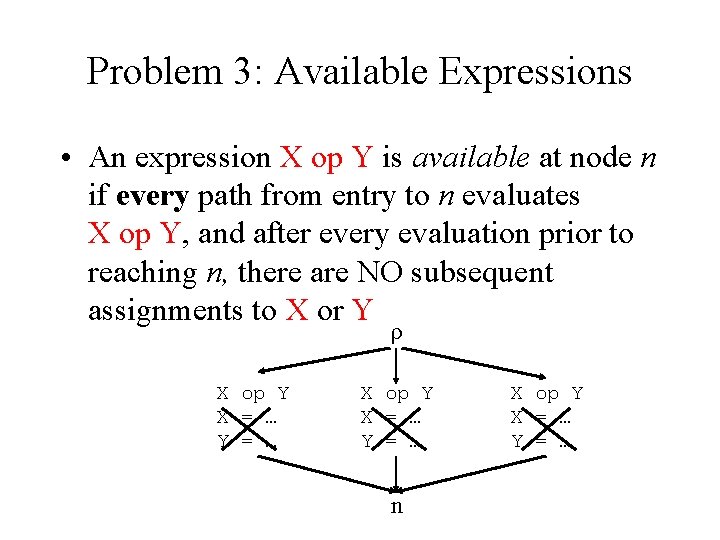
Problem 3: Available Expressions • An expression X op Y is available at node n if every path from entry to n evaluates X op Y, and after every evaluation prior to reaching n, there are NO subsequent assignments to X or Y ρ X op Y X = … Y = … n X op Y X = … Y = …

Global Common Subexpressions z=a*b r=2*z q=a*b u=a*b z=u/2 w=a*b

Global Common Subexpressions t 1=a*b z=t 1 r=2*z t 1=a*b q=t 1 u=t 1 z=u/2 w=a*b Can we eliminate w=a*b?

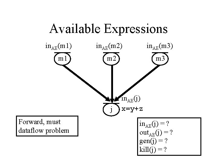
Available Expressions in. AE(m 1) m 1 in. AE(m 2) m 2 j Forward, must dataflow problem in. AE(m 3) m 3 in. AE(j) x=y+z in. AE(j) = ? out. AE(j) = ? gen(j) = ? kill(j) = ?

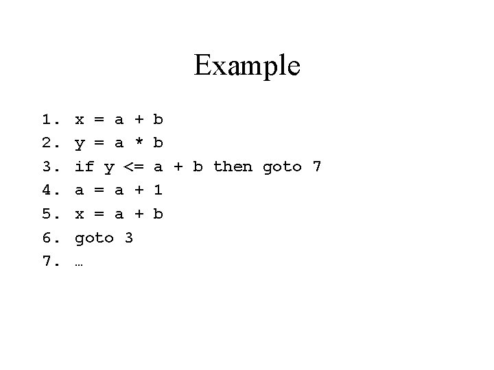
Example 1. 2. 3. 4. 5. 6. 7. x = a + y = a * if y <= a + x = a + goto 3 … b b a + b then goto 7 1 b

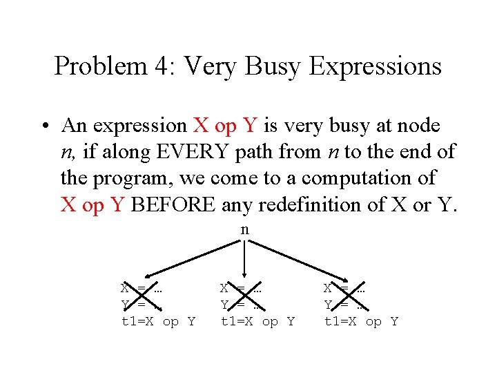
Problem 4: Very Busy Expressions • An expression X op Y is very busy at node n, if along EVERY path from n to the end of the program, we come to a computation of X op Y BEFORE any redefinition of X or Y. n X = … Y = … t 1=X op Y

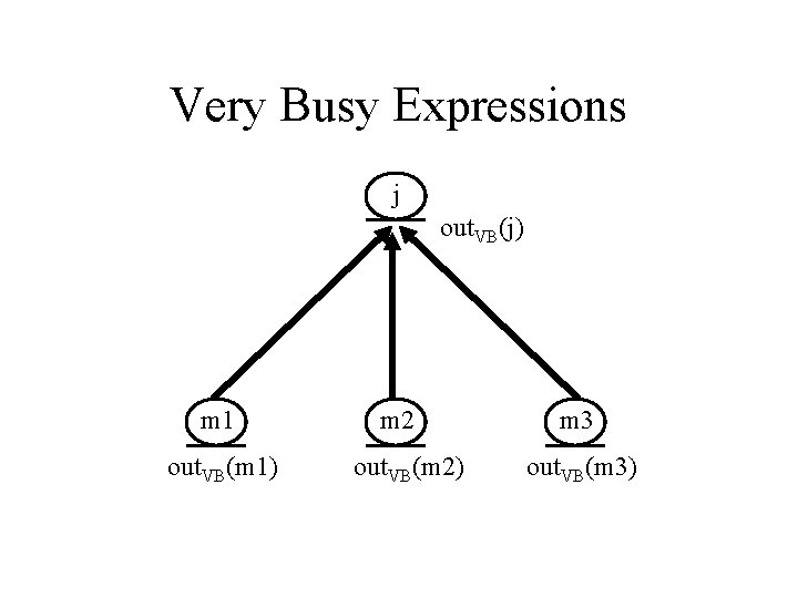
Very Busy Expressions j out. VB(j) m 1 out. VB(m 1) m 2 out. VB(m 2) m 3 out. VB(m 3)

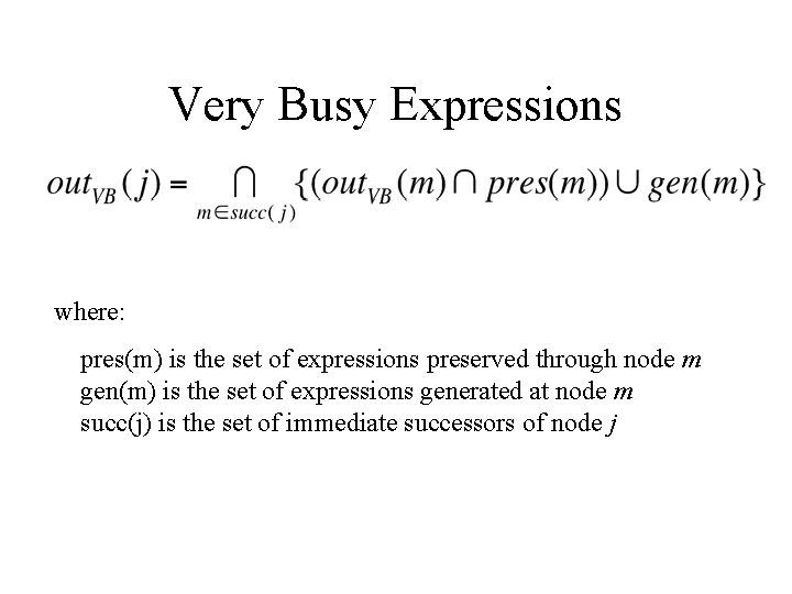
Very Busy Expressions where: pres(m) is the set of expressions preserved through node m gen(m) is the set of expressions generated at node m succ(j) is the set of immediate successors of node j

Dataflow Problems May Problems Must Problems Forward Problems Reaching Definitions Available Expressions Backward Problems Live Uses of Variables Very Busy Expressions

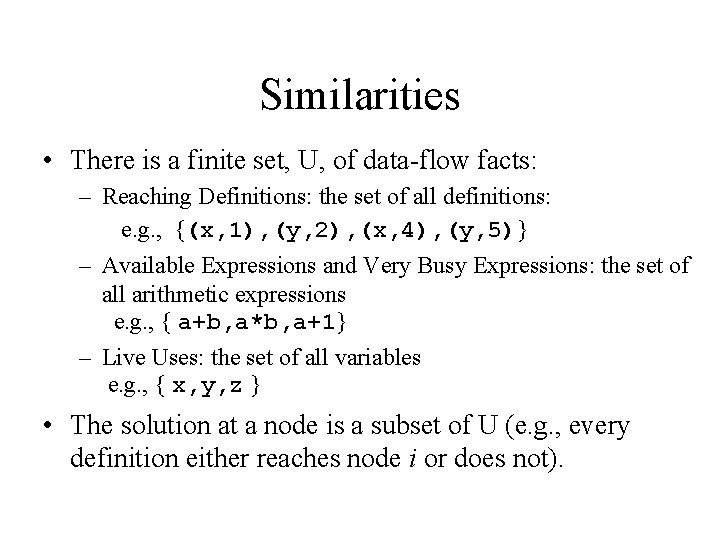
Similarities • There is a finite set, U, of data-flow facts: – Reaching Definitions: the set of all definitions: e. g. , {(x, 1), (y, 2), (x, 4), (y, 5)} – Available Expressions and Very Busy Expressions: the set of all arithmetic expressions e. g. , { a+b, a*b, a+1} – Live Uses: the set of all variables e. g. , { x, y, z } • The solution at a node is a subset of U (e. g. , every definition either reaches node i or does not).

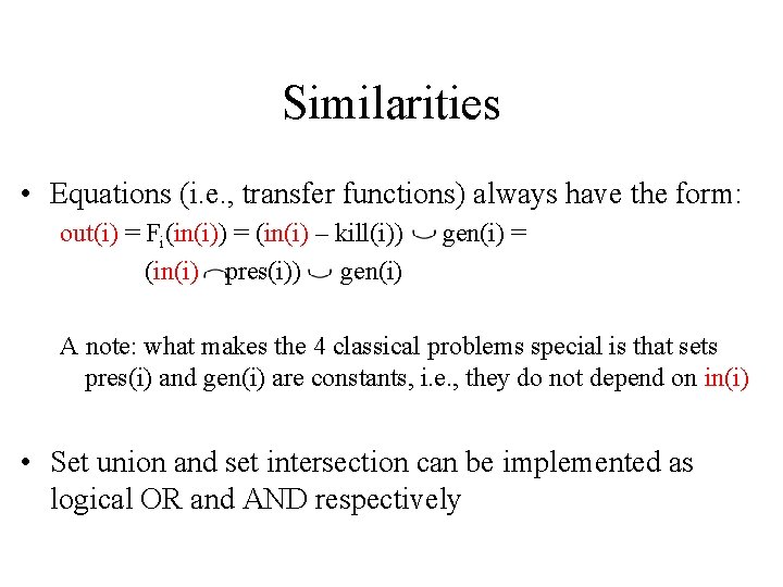
Similarities • Equations (i. e. , transfer functions) always have the form: out(i) = Fi(in(i)) = (in(i) – kill(i)) (in(i) pres(i)) gen(i) = A note: what makes the 4 classical problems special is that sets pres(i) and gen(i) are constants, i. e. , they do not depend on in(i) • Set union and set intersection can be implemented as logical OR and AND respectively

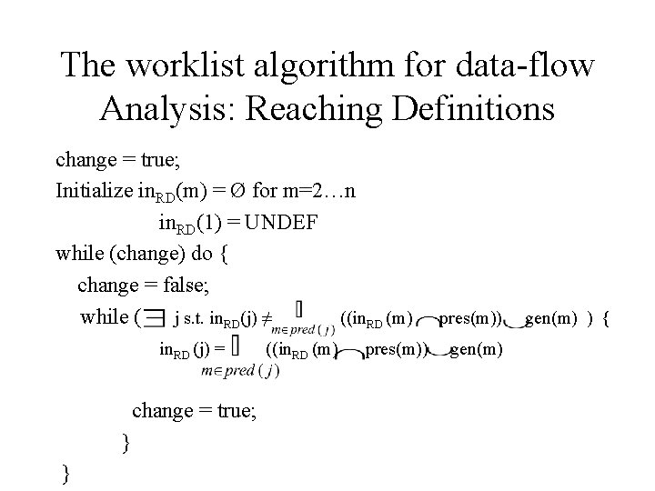
The worklist algorithm for data-flow Analysis: Reaching Definitions change = true; Initialize in. RD(m) = Ø for m=2…n in. RD(1) = UNDEF while (change) do { change = false; while ( j s. t. in. RD(j) ≠ ((in. RD (m) in. RD (j) = change = true; } } ((in. RD (m) pres(m)) gen(m) ) {

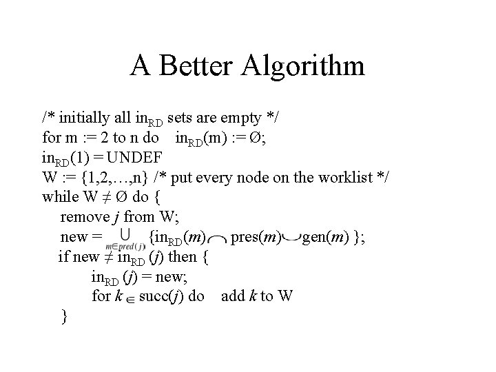
A Better Algorithm /* initially all in. RD sets are empty */ for m : = 2 to n do in. RD(m) : = Ø; in. RD(1) = UNDEF W : = {1, 2, …, n} /* put every node on the worklist */ while W ≠ Ø do { remove j from W; new = {in. RD(m) pres(m) gen(m) }; if new ≠ in. RD (j) then { in. RD (j) = new; for k succ(j) do add k to W }

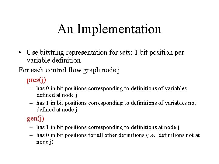
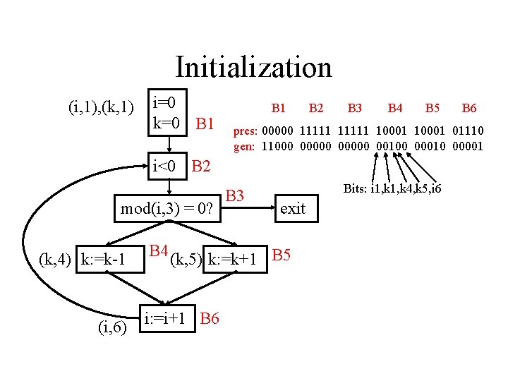
An Implementation • Use bitstring representation for sets: 1 bit position per variable definition For each control flow graph node j pres(j) – has 0 in bit positions corresponding to definitions of variables defined at node j – has 1 in bit positions corresponding to definitions of variables not defined at node j gen(j) – has 1 in bit positions corresponding to definitions at node j – has 0 in bit positions for all other definitions (i. e. , definitions not at node j)

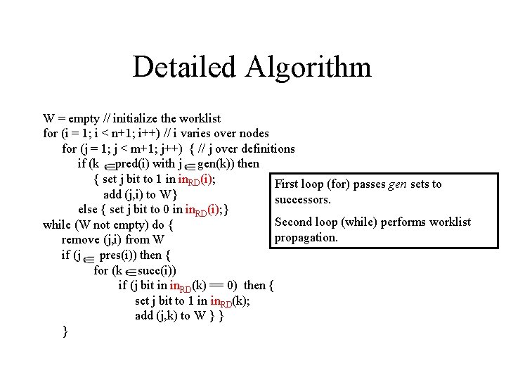
Detailed Algorithm W = empty // initialize the worklist for (i = 1; i < n+1; i++) // i varies over nodes for (j = 1; j < m+1; j++) { // j over definitions if (k pred(i) with j gen(k)) then { set j bit to 1 in in. RD(i); First loop (for) passes gen sets to add (j, i) to W} successors. else { set j bit to 0 in in. RD(i); } Second loop (while) performs worklist while (W not empty) do { propagation. remove (j, i) from W if (j pres(i)) then { for (k succ(i)) if (j bit in in. RD(k) == 0) then { set j bit to 1 in in. RD(k); add (j, k) to W } } }

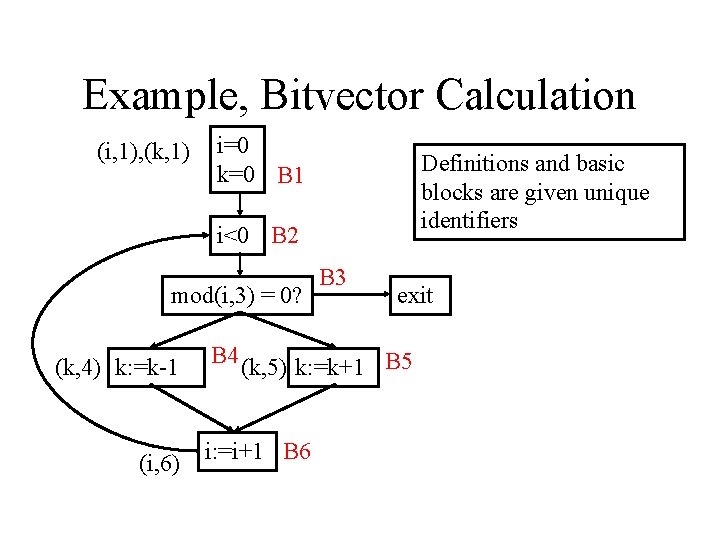
Example, Bitvector Calculation (i, 1), (k, 1) i=0 k=0 B 1 Definitions and basic blocks are given unique identifiers i<0 B 2 mod(i, 3) = 0? (k, 4) k: =k-1 (i, 6) B 3 exit B 4 (k, 5) k: =k+1 B 5 i: =i+1 B 6

Initialization (i, 1), (k, 1) i=0 k=0 B 1 B 2 B 3 B 4 B 5 pres: 00000 11111 10001 01110 gen: 11000 00000 00100 00010 00001 i<0 B 2 mod(i, 3) = 0? (k, 4) k: =k-1 (i, 6) B 3 Bits: i 1, k 4, k 5, i 6 exit B 4 (k, 5) k: =k+1 B 5 i: =i+1 B 6

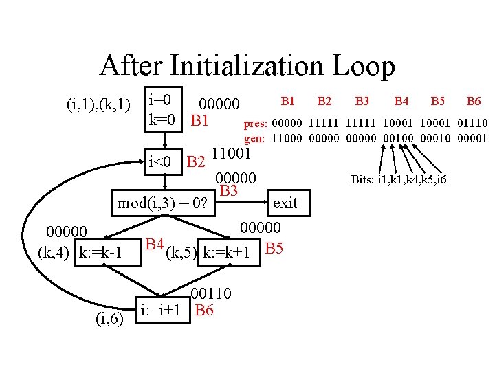
After Initialization Loop (i, 1), (k, 1) i=0 B 1 00000 k=0 B 1 pres: 00000 B 2 B 3 B 4 B 5 B 6 11111 10001 01110 gen: 11000 00000 00100 00010 00001 i<0 B 2 11001 00000 B 3 mod(i, 3) = 0? exit 00000 (k, 4) k: =k-1 B 4 (k, 5) k: =k+1 B 5 (i, 6) 00110 i: =i+1 B 6 Bits: i 1, k 4, k 5, i 6

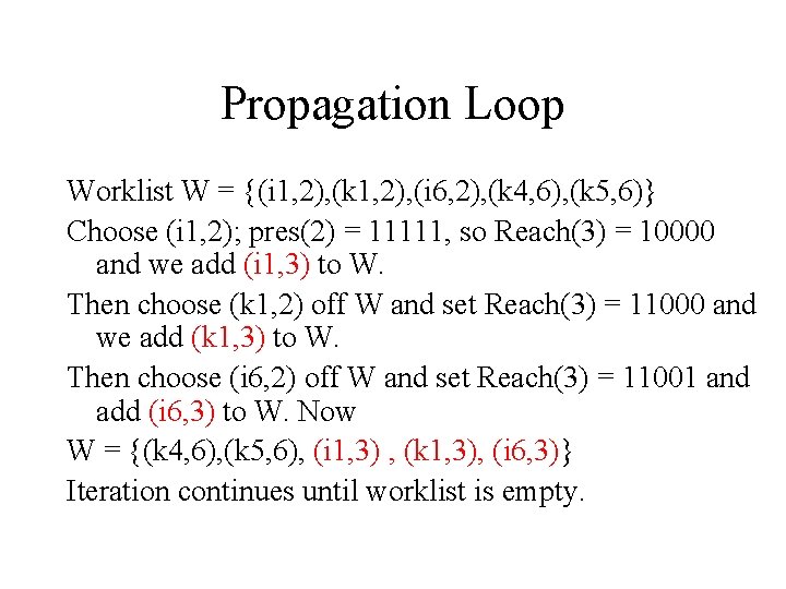
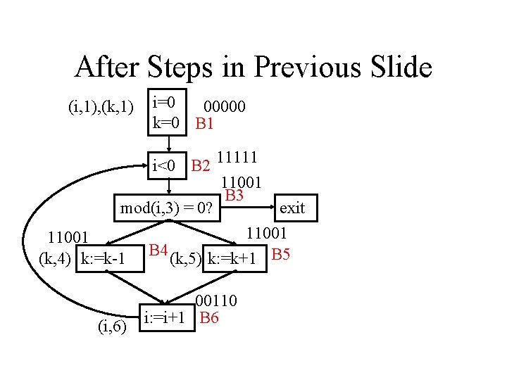
Propagation Loop Worklist W = {(i 1, 2), (k 1, 2), (i 6, 2), (k 4, 6), (k 5, 6)} Choose (i 1, 2); pres(2) = 11111, so Reach(3) = 10000 and we add (i 1, 3) to W. Then choose (k 1, 2) off W and set Reach(3) = 11000 and we add (k 1, 3) to W. Then choose (i 6, 2) off W and set Reach(3) = 11001 and add (i 6, 3) to W. Now W = {(k 4, 6), (k 5, 6), (i 1, 3) , (k 1, 3), (i 6, 3)} Iteration continues until worklist is empty.

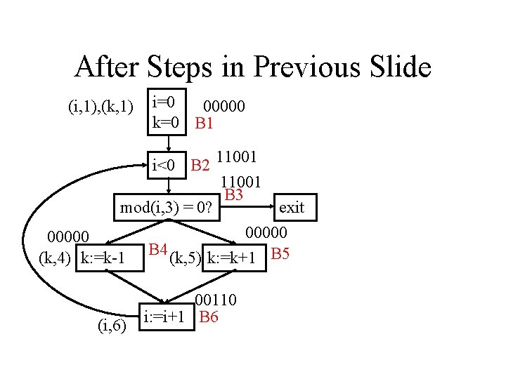
After Steps in Previous Slide (i, 1), (k, 1) i=0 00000 k=0 B 1 i<0 B 2 11001 B 3 mod(i, 3) = 0? exit 00000 (k, 4) k: =k-1 B 4 (k, 5) k: =k+1 B 5 (i, 6) 00110 i: =i+1 B 6

After Steps in Previous Slide (i, 1), (k, 1) i=0 00000 k=0 B 1 i<0 B 2 11111 11001 B 3 mod(i, 3) = 0? exit 00000 (k, 4) k: =k-1 B 4 (k, 5) k: =k+1 B 5 (i, 6) 00110 i: =i+1 B 6

After Steps in Previous Slide (i, 1), (k, 1) i=0 00000 k=0 B 1 i<0 B 2 11111 11001 B 3 mod(i, 3) = 0? exit 11001 (k, 4) k: =k-1 B 4 (k, 5) k: =k+1 B 5 (i, 6) 00110 i: =i+1 B 6

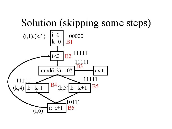
Solution (skipping some steps) (i, 1), (k, 1) i=0 00000 k=0 B 1 i<0 B 2 11111 B 3 mod(i, 3) = 0? exit 11111 (k, 4) k: =k-1 B 4 (k, 5) k: =k+1 B 5 (i, 6) 10111 i: =i+1 B 6