Course Outline Traditional Static Program Analysis Theory Compiler

Course Outline • Traditional Static Program Analysis – Theory • Compiler Optimizations; Control Flow Graphs • Data-flow Analysis – today’s class – Classic analyses and applications • Software Testing • Dynamic Program Analysis

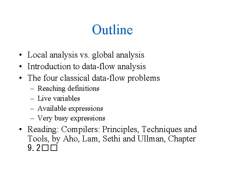
Outline • Local analysis vs. global analysis • Introduction to data-flow analysis • The four classical data-flow problems – – Reaching definitions Live variables Available expressions Very busy expressions • Reading: Compilers: Principles, Techniques and Tools, by Aho, Lam, Sethi and Ullman, Chapter 9. 2��

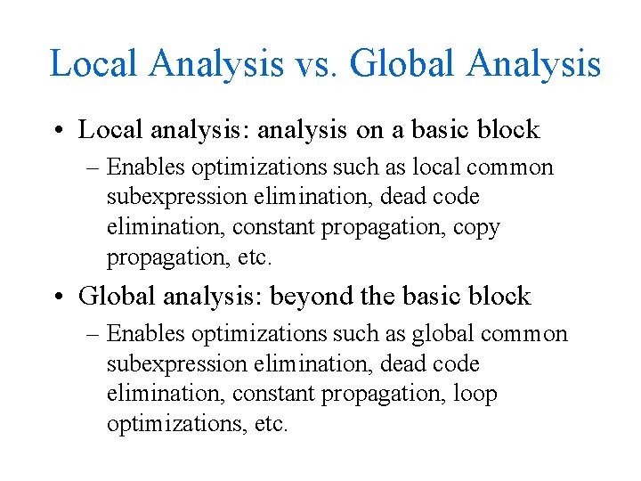
Local Analysis vs. Global Analysis • Local analysis: analysis on a basic block – Enables optimizations such as local common subexpression elimination, dead code elimination, constant propagation, copy propagation, etc. • Global analysis: beyond the basic block – Enables optimizations such as global common subexpression elimination, dead code elimination, constant propagation, loop optimizations, etc.

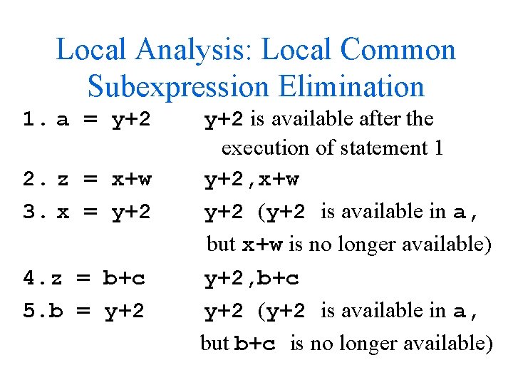
Local Analysis: Local Common Subexpression Elimination 1. a = y+2 2. z = x+w 3. x = y+2 4. z = b+c 5. b = y+2 is available after the execution of statement 1 y+2, x+w y+2 (y+2 is available in a, but x+w is no longer available) y+2, b+c y+2 (y+2 is available in a, but b+c is no longer available)

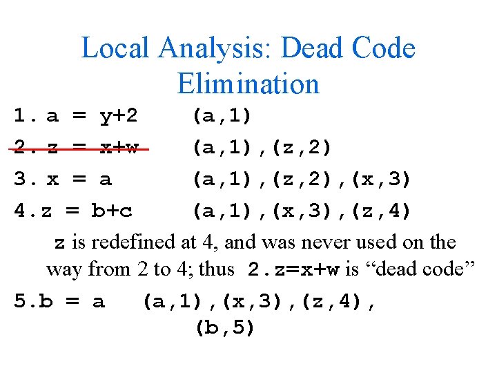
Local Analysis: Dead Code Elimination 1. a = y+2 (a, 1) 2. z = x+w (a, 1), (z, 2) 3. x = a (a, 1), (z, 2), (x, 3) 4. z = b+c (a, 1), (x, 3), (z, 4) z is redefined at 4, and was never used on the way from 2 to 4; thus 2. z=x+w is “dead code” 5. b = a (a, 1), (x, 3), (z, 4), (b, 5)

Local Analysis vs. Global Analysis • Local analysis is easy – we need to take into account a single path, from basic block entry to basic block exit • Global analysis is harder – we need to take into account multiple paths, across basic blocks

Introduction to Data-flow Analysis • Collects information about the flow of data along execution paths� – Loops (control goes back) – Control splits and control merges • Data-flow information • Data-flow analysis

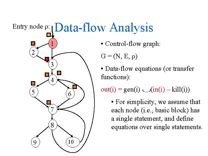
Data-flow Analysis Entry node ρ: • Control-flow graph: 1 2 G = (N, E, ρ) 3 • Data-flow equations (or transfer functions): 4 5 6 (in(i) – kill(i)) • For simplicity, we assume that each node (i. e. , basic block) has a single statement, and define equations over single statements. 7 8 9 out(i) = gen(i) 10

Four Classical Data-flow Problems • • • Reaching definitions (Reach) Live uses of variables (Live) Available expressions (Avail) Very busy expressions (Very. B) Def-use chains built from Reach, and the dual Use -def chains, built from Live, play role in many optimizations • Avail enables global common subexpression elimination • Very. B is used for conservative code motion

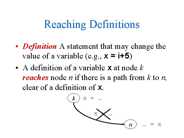
Reaching Definitions • Definition A statement that may change the value of a variable (e. g. , x = i+5) • A definition of a variable x at node k reaches node n if there is a path from k to n, clear of a definition of x. k x = … n … = x

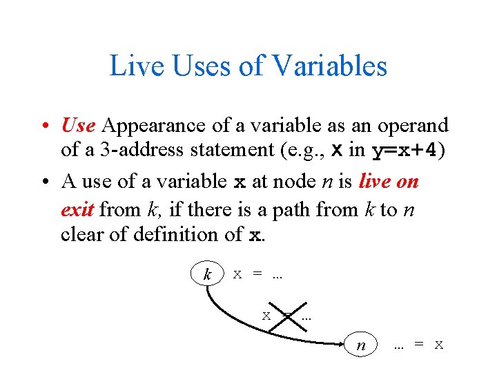
Live Uses of Variables • Use Appearance of a variable as an operand of a 3 -address statement (e. g. , x in y=x+4) • A use of a variable x at node n is live on exit from k, if there is a path from k to n clear of definition of x. k x = … n … = x

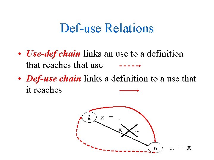
Def-use Relations • Use-def chain links an use to a definition that reaches that use • Def-use chain links a definition to a use that it reaches k x = … n … = x

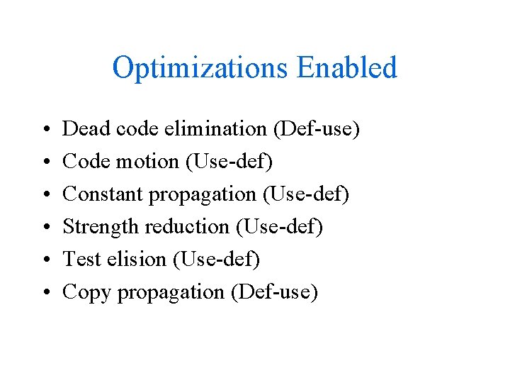
Optimizations Enabled • • • Dead code elimination (Def-use) Code motion (Use-def) Constant propagation (Use-def) Strength reduction (Use-def) Test elision (Use-def) Copy propagation (Def-use)

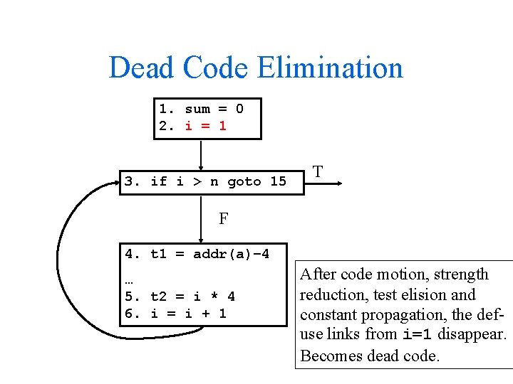
Dead Code Elimination 1. sum = 0 2. i = 1 3. if i > n goto 15 T F 4. t 1 = addr(a)– 4 … 5. t 2 = i * 4 6. i = i + 1 After code motion, strength reduction, test elision and constant propagation, the defuse links from i=1 disappear. Becomes dead code.

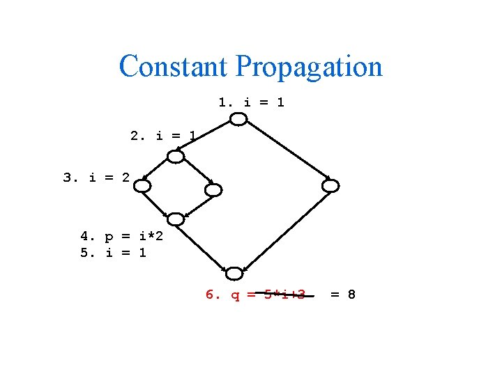
Constant Propagation 1. i = 1 2. i = 1 3. i = 2 4. p = i*2 5. i = 1 6. q = 5*i+3 = 8

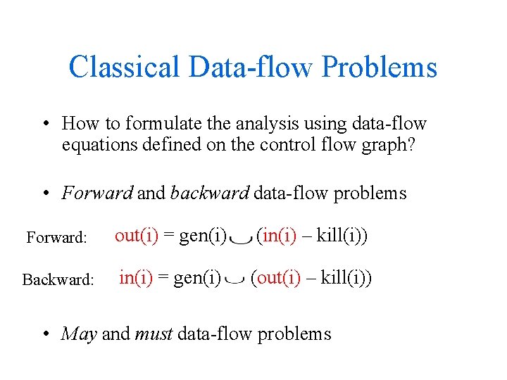
Classical Data-flow Problems • How to formulate the analysis using data-flow equations defined on the control flow graph? • Forward and backward data-flow problems Forward: out(i) = gen(i) (in(i) – kill(i)) Backward: in(i) = gen(i) (out(i) – kill(i)) • May and must data-flow problems

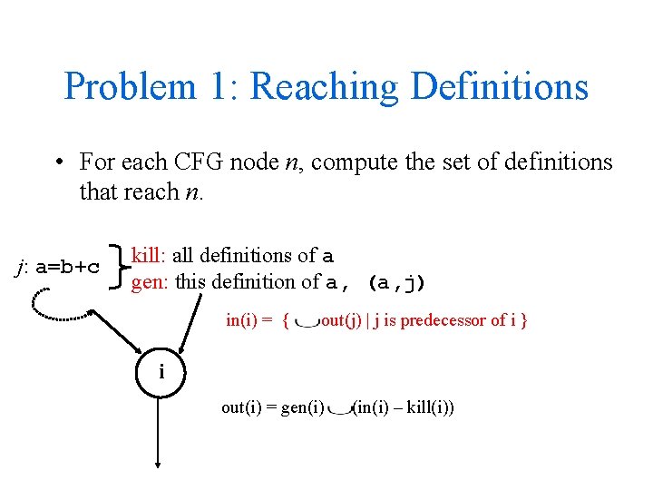
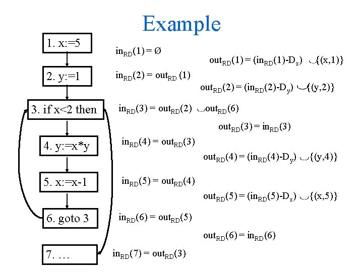
Problem 1: Reaching Definitions • For each CFG node n, compute the set of definitions that reach n. j: a=b+c kill: all definitions of a gen: this definition of a, (a, j) in(i) = { out(j) | j is predecessor of i } i out(i) = gen(i) (in(i) – kill(i))

Example 1. x: =5 in. RD(1) = Ø 2. y: =1 in. RD(2) = out. RD (1) 3. if x<2 then in. RD(3) = out. RD(2) out. RD(1) = (in. RD(1)-Dx) out. RD(2) = (in. RD(2)-Dy) {(x, 1)} {(y, 2)} out. RD(6) out. RD(3) = in. RD(3) 4. y: =x*y in. RD(4) = out. RD(3) 5. x: =x-1 in. RD(5) = out. RD(4) 6. goto 3 out. RD(4) = (in. RD(4)-Dy) {(y, 4)} out. RD(5) = (in. RD(5)-Dx) {(x, 5)} in. RD(6) = out. RD(5) out. RD(6) = in. RD(6) 7. … in. RD(7) = out. RD(3)

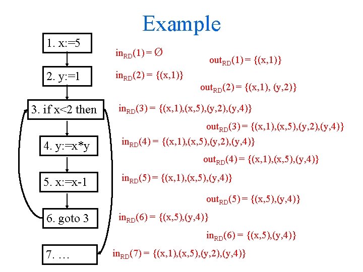
Example 1. x: =5 2. y: =1 3. if x<2 then in. RD(1) = Ø in. RD(2) = {(x, 1)} out. RD(1) = {(x, 1)} out. RD(2) = {(x, 1), (y, 2)} in. RD(3) = {(x, 1), (x, 5), (y, 2), (y, 4)} out. RD(3) = {(x, 1), (x, 5), (y, 2), (y, 4)} 4. y: =x*y in. RD(4) = {(x, 1), (x, 5), (y, 2), (y, 4)} out. RD(4) = {(x, 1), (x, 5), (y, 4)} 5. x: =x-1 in. RD(5) = {(x, 1), (x, 5), (y, 4)} out. RD(5) = {(x, 5), (y, 4)} 6. goto 3 in. RD(6) = {(x, 5), (y, 4)} 7. … in. RD(7) = {(x, 1), (x, 5), (y, 2), (y, 4)}

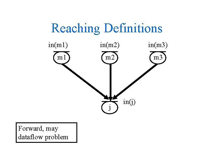
Reaching Definitions in(m 1) m 1 in(m 2) in(m 3) m 2 m 3 j Forward, may dataflow problem in(j)

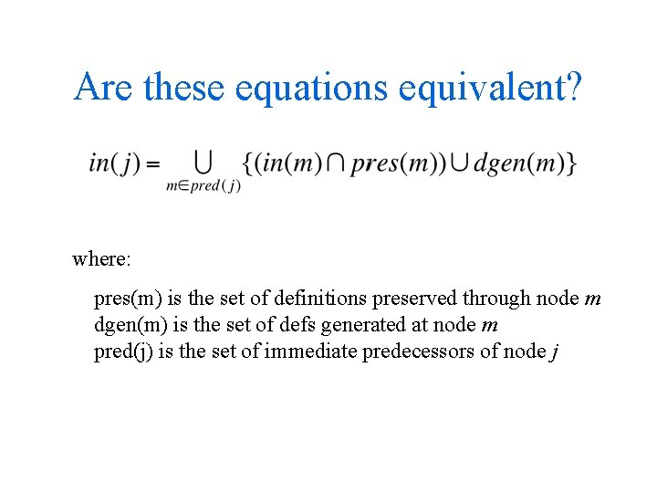
Are these equations equivalent? where: pres(m) is the set of definitions preserved through node m dgen(m) is the set of defs generated at node m pred(j) is the set of immediate predecessors of node j

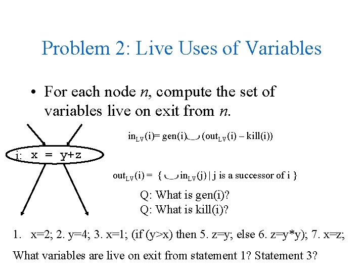
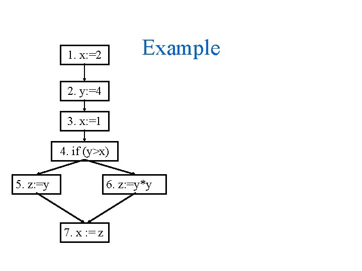
Problem 2: Live Uses of Variables • For each node n, compute the set of variables live on exit from n. in. LV(i)= gen(i) (out. LV(i) – kill(i)) i: x = y+z out. LV(i) = { in. LV(j) | j is a successor of i } Q: What is gen(i)? Q: What is kill(i)? 1. x=2; 2. y=4; 3. x=1; (if (y>x) then 5. z=y; else 6. z=y*y); 7. x=z; What variables are live on exit from statement 1? Statement 3?

Example 1. x: =2 2. y: =4 3. x: =1 4. if (y>x) 5. z: =y 6. z: =y*y 7. x : = z

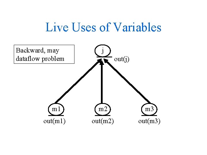
Live Uses of Variables Backward, may dataflow problem j out(j) m 1 m 2 m 3 out(m 1) out(m 2) out(m 3)

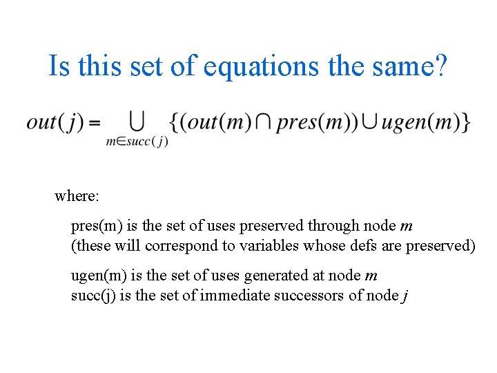
Is this set of equations the same? where: pres(m) is the set of uses preserved through node m (these will correspond to variables whose defs are preserved) ugen(m) is the set of uses generated at node m succ(j) is the set of immediate successors of node j

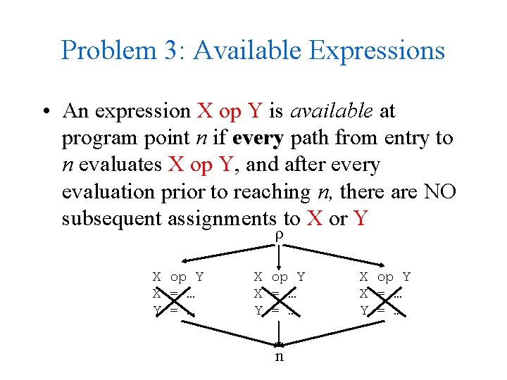
Problem 3: Available Expressions • An expression X op Y is available at program point n if every path from entry to n evaluates X op Y, and after every evaluation prior to reaching n, there are NO subsequent assignments to X or Y ρ X op Y X = … Y = … n X op Y X = … Y = …

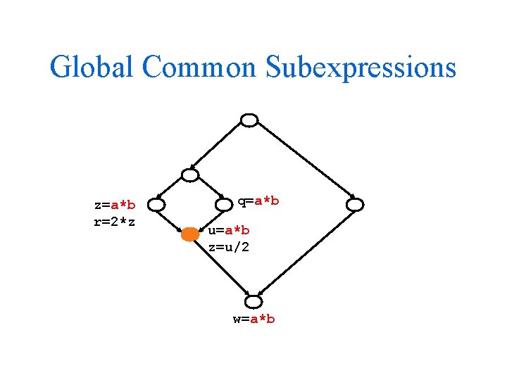
Global Common Subexpressions z=a*b r=2*z q=a*b u=a*b z=u/2 w=a*b

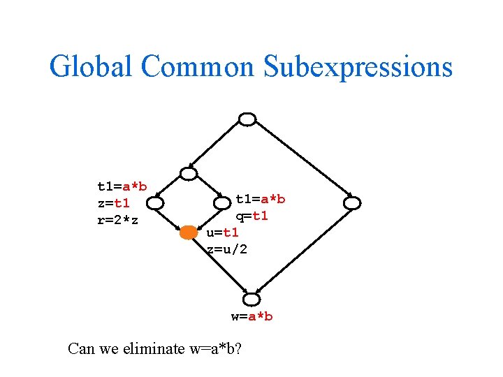
Global Common Subexpressions t 1=a*b z=t 1 r=2*z t 1=a*b q=t 1 u=t 1 z=u/2 w=a*b Can we eliminate w=a*b?

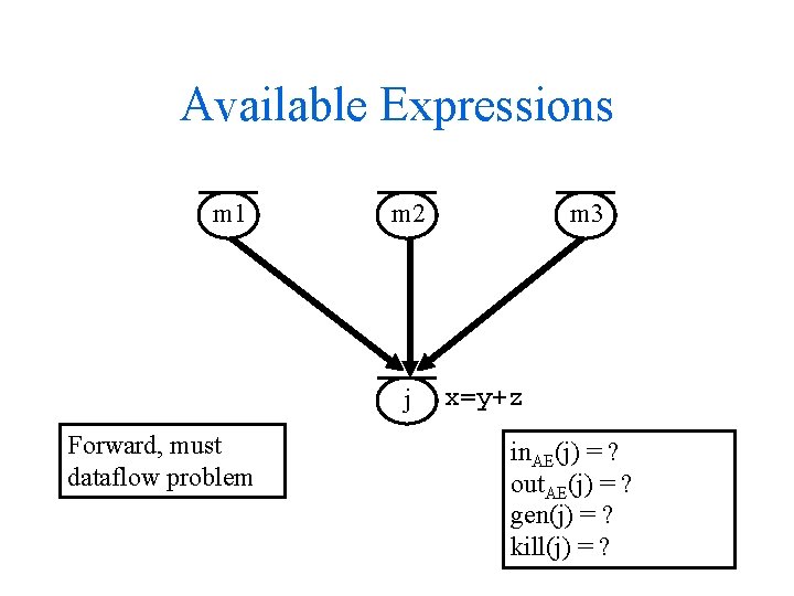
Available Expressions m 1 m 2 j Forward, must dataflow problem m 3 x=y+z in. AE(j) = ? out. AE(j) = ? gen(j) = ? kill(j) = ?

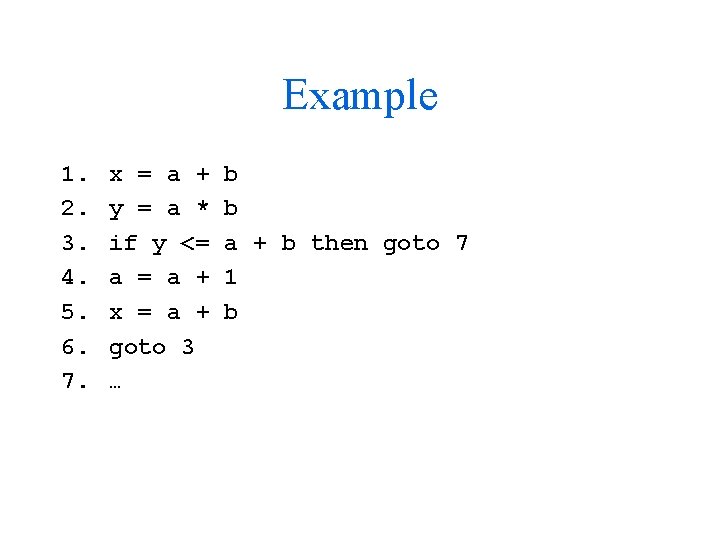
Example 1. 2. 3. 4. 5. 6. 7. x = a + y = a * if y <= a + x = a + goto 3 … b b a + b then goto 7 1 b

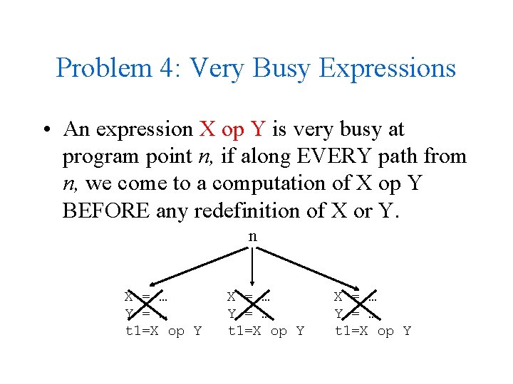
Problem 4: Very Busy Expressions • An expression X op Y is very busy at program point n, if along EVERY path from n, we come to a computation of X op Y BEFORE any redefinition of X or Y. n X = … Y = … t 1=X op Y

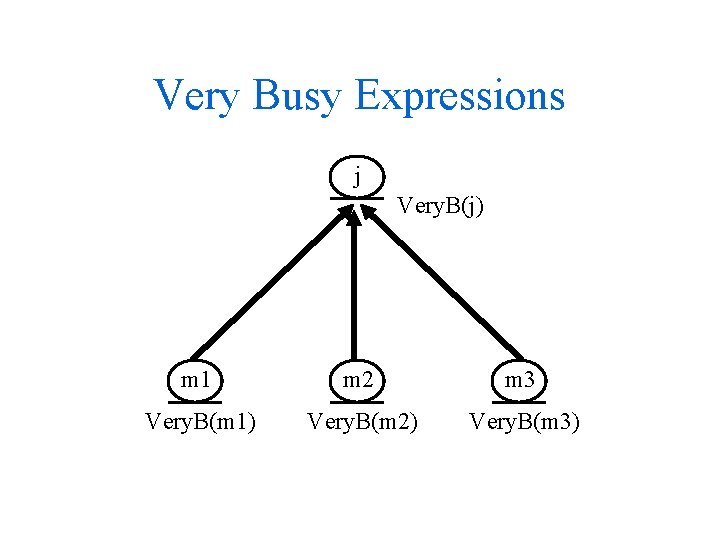
Very Busy Expressions j Very. B(j) m 1 m 2 m 3 Very. B(m 1) Very. B(m 2) Very. B(m 3)

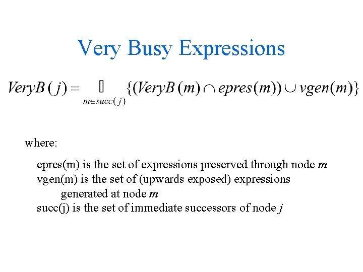
Very Busy Expressions where: epres(m) is the set of expressions preserved through node m vgen(m) is the set of (upwards exposed) expressions generated at node m succ(j) is the set of immediate successors of node j

Terms • • • Data-flow Analysis Reaching Definitions Live Variables Available Expressions Very Busy Expressions • (More later) May-problem, Must problem, Forward problem, Backward problem