Course Outline Traditional Static Program Analysis Theory Compiler

Course Outline • Traditional Static Program Analysis – Theory • Compiler Optimizations; Control Flow Graphs, • Data-flow Analysis • Data-flow Frameworks --- today’s class – Specific Analyses, Applications, etc. • Software Testing • Dynamic Program Analysis

Announcement • Handout • Homework 1, due February 17 th

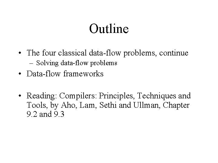
Outline • The four classical data-flow problems, continue – Solving data-flow problems • Data-flow frameworks • Reading: Compilers: Principles, Techniques and Tools, by Aho, Lam, Sethi and Ullman, Chapter 9. 2 and 9. 3

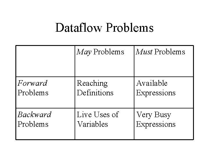
Dataflow Problems May Problems Must Problems Forward Problems Reaching Definitions Available Expressions Backward Problems Live Uses of Variables Very Busy Expressions

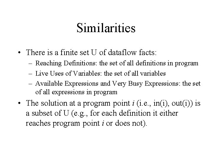
Similarities • There is a finite set U of dataflow facts: – Reaching Definitions: the set of all definitions in program – Live Uses of Variables: the set of all variables – Available Expressions and Very Busy Expressions: the set of all expressions in program • The solution at a program point i (i. e. , in(i), out(i)) is a subset of U (e. g. , for each definition it either reaches program point i or does not).

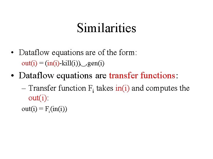
Similarities • Dataflow equations are of the form: out(i) = (in(i)-kill(i)) gen(i) • Dataflow equations are transfer functions: – Transfer function Fi takes in(i) and computes the out(i): out(i) = Fi(in(i))

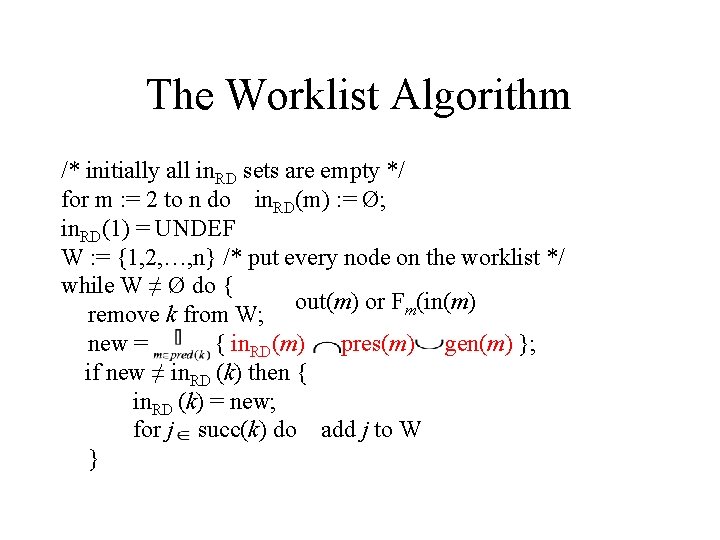
The Worklist Algorithm /* initially all in. RD sets are empty */ for m : = 2 to n do in. RD(m) : = Ø; in. RD(1) = UNDEF W : = {1, 2, …, n} /* put every node on the worklist */ while W ≠ Ø do { out(m) or Fm(in(m) remove k from W; new = { in. RD(m) pres(m) gen(m) }; if new ≠ in. RD (k) then { in. RD (k) = new; for j succ(k) do add j to W }

Dataflow Frameworks • Lattices – Partial ordering – Meet, Join, Lattice, and Chain • Monotone functions • The “Maximal Fixed Point” (MFP) solution • The “Meet Over all Paths” (MOP) solution

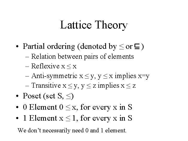
Lattice Theory • Partial ordering (denoted by ≤ or ) – Relation between pairs of elements – Reflexive x ≤ x – Anti-symmetric x ≤ y, y ≤ x implies x=y – Transitive x ≤ y, y ≤ z implies x ≤ z • Poset (set S, ≤) • 0 Element 0 ≤ x, for every x in S • 1 Element x ≤ 1, for every x in S We don’t necessarily need 0 and 1 element.

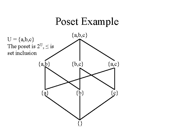
Poset Example U = {a, b, c} The poset is 2 U, ≤ is set inclusion {a, b, c} {a, b} {b, c} {a} {b} {c} {}

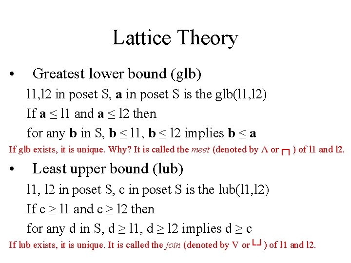
Lattice Theory • Greatest lower bound (glb) l 1, l 2 in poset S, a in poset S is the glb(l 1, l 2) If a ≤ l 1 and a ≤ l 2 then for any b in S, b ≤ l 1, b ≤ l 2 implies b ≤ a If glb exists, it is unique. Why? It is called the meet (denoted by Λ or┌┐) of l 1 and l 2. • Least upper bound (lub) l 1, l 2 in poset S, c in poset S is the lub(l 1, l 2) If c ≥ l 1 and c ≥ l 2 then for any d in S, d ≥ l 1, d ≥ l 2 implies d ≥ c If lub exists, it is unique. It is called the join (denoted by V or└┘) of l 1 and l 2.

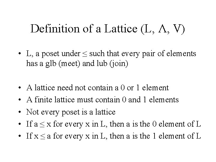
Definition of a Lattice (L, Λ, V) • L, a poset under ≤ such that every pair of elements has a glb (meet) and lub (join) • • • A lattice need not contain a 0 or 1 element A finite lattice must contain 0 and 1 elements Not every poset is a lattice If a ≤ x for every x in L, then a is the 0 element of L If x ≤ a for every x in L, then a is the 1 element of L

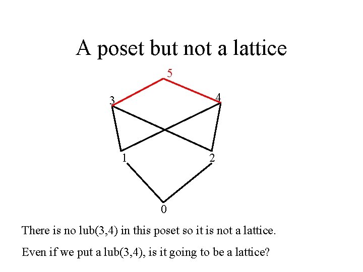
A poset but not a lattice 5 4 3 1 2 0 There is no lub(3, 4) in this poset so it is not a lattice. Even if we put a lub(3, 4), is it going to be a lattice?

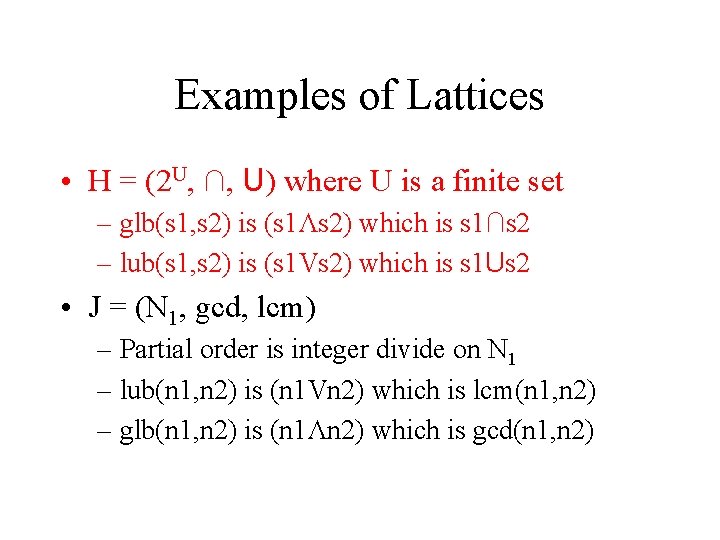
Examples of Lattices • H = (2 U, ∩, U) where U is a finite set – glb(s 1, s 2) is (s 1Λs 2) which is s 1∩s 2 – lub(s 1, s 2) is (s 1 Vs 2) which is s 1 Us 2 • J = (N 1, gcd, lcm) – Partial order is integer divide on N 1 – lub(n 1, n 2) is (n 1 Vn 2) which is lcm(n 1, n 2) – glb(n 1, n 2) is (n 1Λn 2) which is gcd(n 1, n 2)

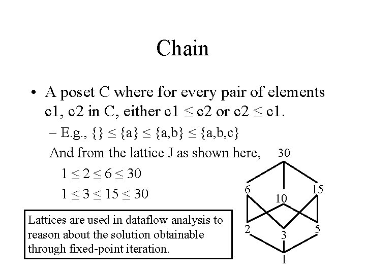
Chain • A poset C where for every pair of elements c 1, c 2 in C, either c 1 ≤ c 2 or c 2 ≤ c 1. – E. g. , {} ≤ {a, b} ≤ {a, b, c} And from the lattice J as shown here, 30 1 ≤ 2 ≤ 6 ≤ 30 6 1 ≤ 3 ≤ 15 ≤ 30 10 Lattices are used in dataflow analysis to reason about the solution obtainable through fixed-point iteration. 2 3 1 15 5

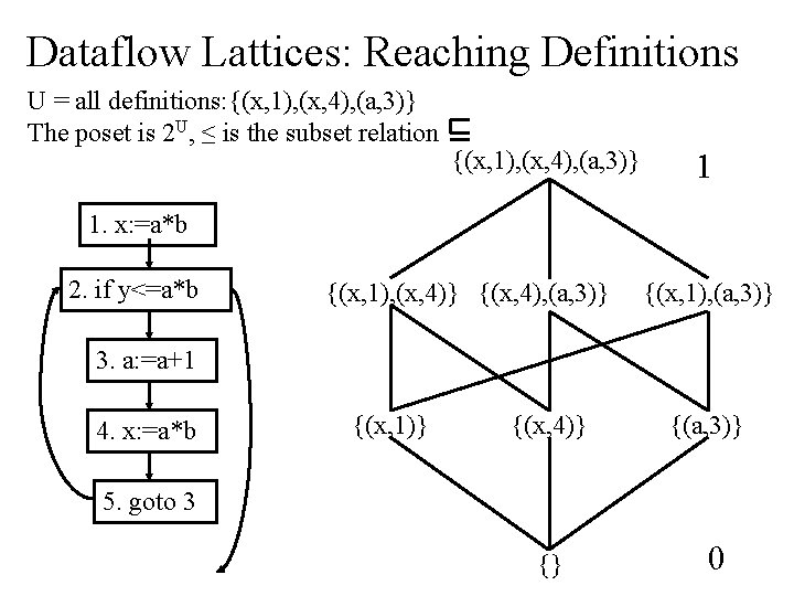
Dataflow Lattices: Reaching Definitions U = all definitions: {(x, 1), (x, 4), (a, 3)} The poset is 2 U, ≤ is the subset relation {(x, 1), (x, 4), (a, 3)} 1 1. x: =a*b 2. if y<=a*b {(x, 1), (x, 4)} {(x, 4), (a, 3)} {(x, 1), (a, 3)} 3. a: =a+1 4. x: =a*b {(x, 1)} {(x, 4)} {(a, 3)} 5. goto 3 {} 0

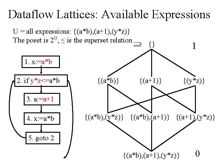
Dataflow Lattices: Available Expressions U = all expressions: {(a*b), (a+1), (y*z)} The poset is 2 U, ≤ is the superset relation {} 1 {(a+1)} {(y*z)} 1. x: =a*b 2. if y*z<=a*b {(a*b)} 3. a: =a+1 4. x: =a*b {(a*b), (y*z)} {(a*b), (a+1)} {(a+1), (y*z)} 5. goto 2 {(a*b), (a+1), (y*z)} 0

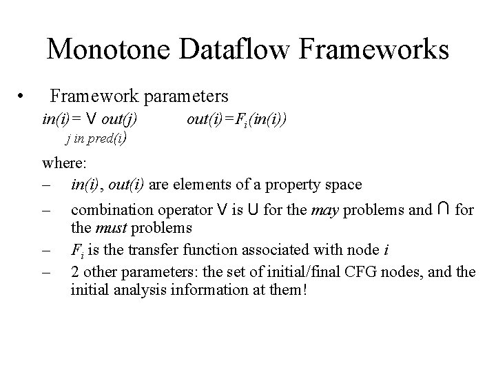
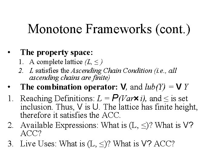
Monotone Dataflow Frameworks • Framework parameters in(i)= V out(j) j in pred(i) out(i)=Fi(in(i)) where: – in(i), out(i) are elements of a property space – – – combination operator V is U for the may problems and ∩ for the must problems Fi is the transfer function associated with node i 2 other parameters: the set of initial/final CFG nodes, and the initial analysis information at them!

Monotone Frameworks (cont. ) • The property space: 1. A complete lattice (L, ≤ ) 2. L satisfies the Ascending Chain Condition (i. e. , all ascending chains are finite) • The combination operator: V, and lub(Y) = V Y 1. Reaching Definitions: L = P(Var i), and ≤ is set inclusion. Thus, V is U. The lattice has finite height, therefore it satisfies the ACC. 2. Available Expressions: What is (L, ≤)? What is V? ACC? 3. Live Uses: What is (L, ≤)? What is V? ACC?

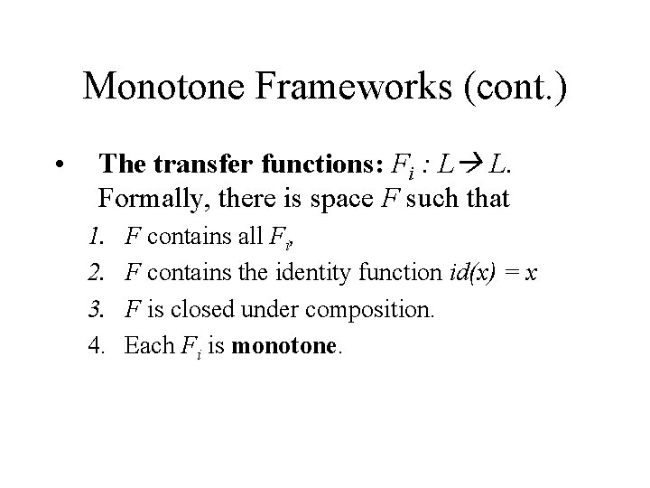
Monotone Frameworks (cont. ) • The transfer functions: Fi : L L. Formally, there is space F such that 1. 2. 3. 4. F contains all Fi, F contains the identity function id(x) = x F is closed under composition. Each Fi is monotone.

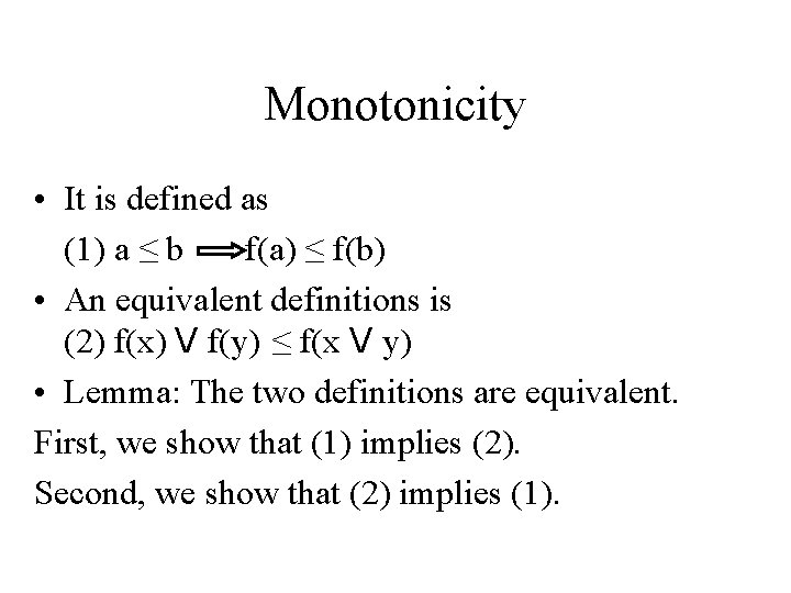
Monotonicity • It is defined as (1) a ≤ b f(a) ≤ f(b) • An equivalent definitions is (2) f(x) V f(y) ≤ f(x V y) • Lemma: The two definitions are equivalent. First, we show that (1) implies (2). Second, we show that (2) implies (1).

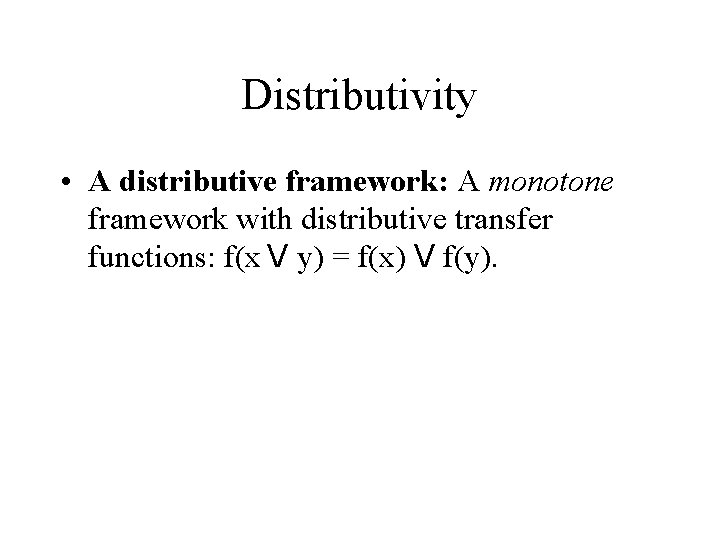
Distributivity • A distributive framework: A monotone framework with distributive transfer functions: f(x V y) = f(x) V f(y).