Correlation Measures the relative strength of the linear

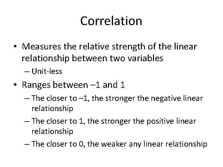
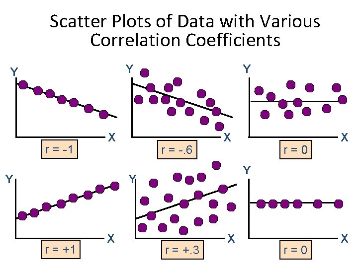
Correlation • Measures the relative strength of the linear relationship between two variables – Unit-less • Ranges between – 1 and 1 – The closer to – 1, the stronger the negative linear relationship – The closer to 1, the stronger the positive linear relationship – The closer to 0, the weaker any linear relationship

Scatter Plots of Data with Various Correlation Coefficients Y Y r = -1 X Y Y r = -. 6 X Y Y r = +1 X r=0 X r = +. 3 X r=0 X

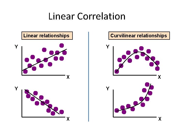
Linear Correlation Linear relationships Y Curvilinear relationships Y X Y X X

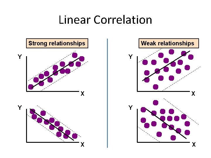
Linear Correlation Strong relationships Y Weak relationships Y X Y X X

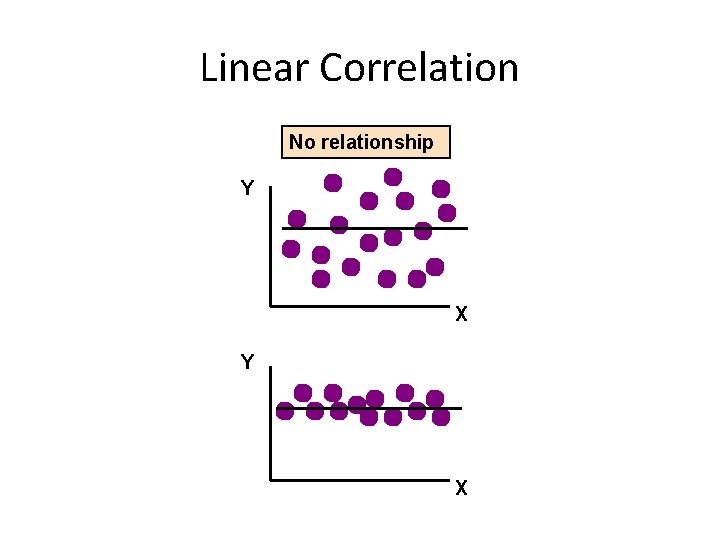
Linear Correlation No relationship Y X

Linear regression • In correlation, the two variables are treated as equals. • In regression, one variable is considered independent (=predictor) variable (X) and the other the dependent (=outcome) variable Y.

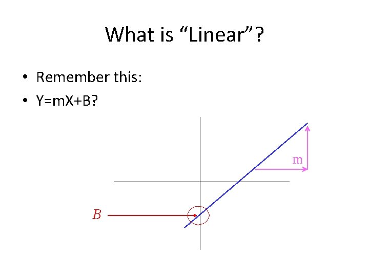
What is “Linear”? • Remember this: • Y=m. X+B? m B

What’s Slope? • A slope of 2 means that every 1 -unit change in X yields a 2 -unit change in Y. • Prediction: • If you know something about X, this knowledge helps you predict something about Y.

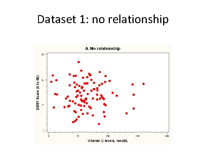
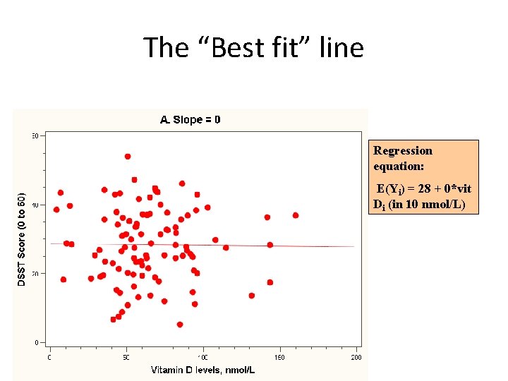
Dataset 1: no relationship

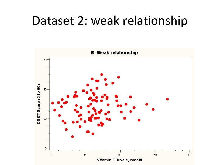
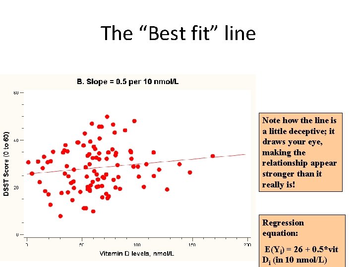
Dataset 2: weak relationship

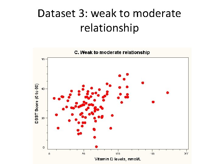
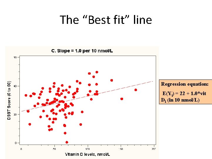
Dataset 3: weak to moderate relationship

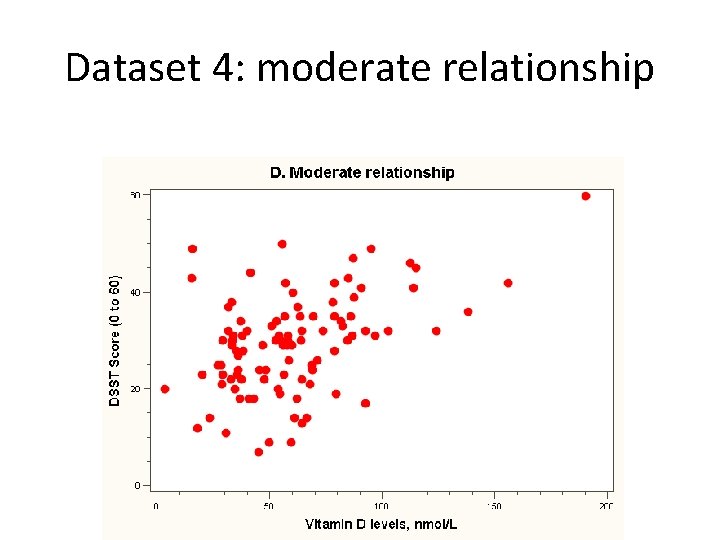
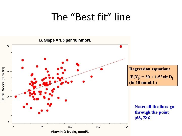
Dataset 4: moderate relationship

The “Best fit” line Regression equation: E(Yi) = 28 + 0*vit Di (in 10 nmol/L)

The “Best fit” line Note how the line is a little deceptive; it draws your eye, making the relationship appear stronger than it really is! Regression equation: E(Yi) = 26 + 0. 5*vit Di (in 10 nmol/L)

The “Best fit” line Regression equation: E(Yi) = 22 + 1. 0*vit Di (in 10 nmol/L)

The “Best fit” line Regression equation: E(Yi) = 20 + 1. 5*vit Di (in 10 nmol/L) Note: all the lines go through the point (63, 28)!

Multiple linear regression… • What if age is a confounder here? – Older men have lower vitamin D – Older men have poorer cognition • “Adjust” for age by putting age in the model: – DSST score = intercept + slope 1 xvitamin D + slope 2 xage

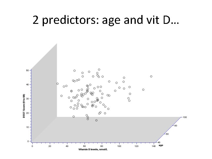
2 predictors: age and vit D…

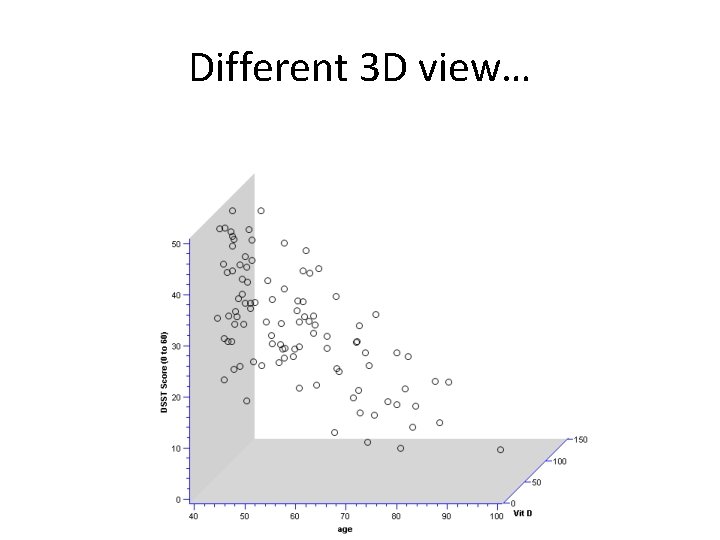
Different 3 D view…

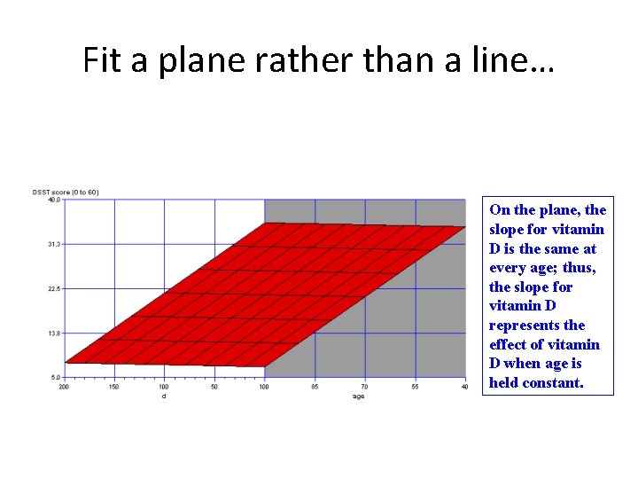
Fit a plane rather than a line… On the plane, the slope for vitamin D is the same at every age; thus, the slope for vitamin D represents the effect of vitamin D when age is held constant.

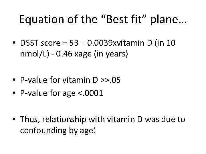
Equation of the “Best fit” plane… • DSST score = 53 + 0. 0039 xvitamin D (in 10 nmol/L) - 0. 46 xage (in years) • P-value for vitamin D >>. 05 • P-value for age <. 0001 • Thus, relationship with vitamin D was due to confounding by age!

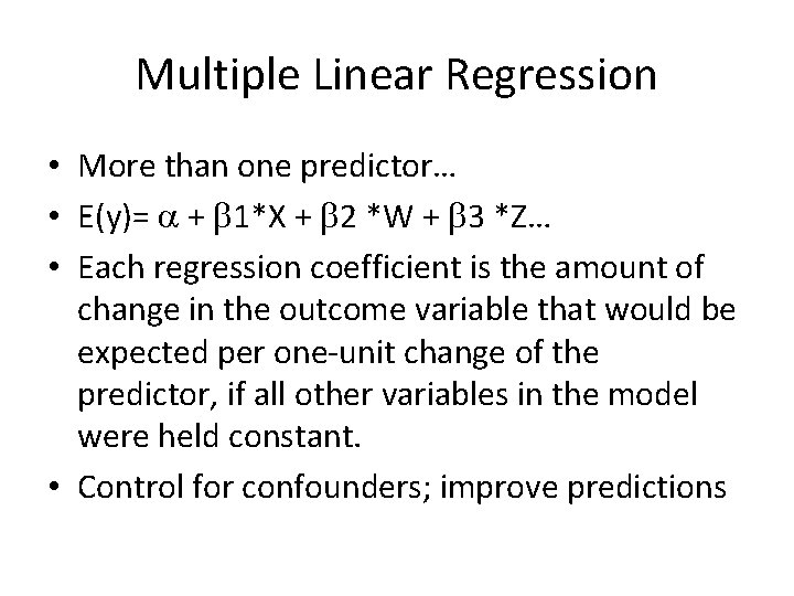
Multiple Linear Regression • More than one predictor… • E(y)= + 1*X + 2 *W + 3 *Z… • Each regression coefficient is the amount of change in the outcome variable that would be expected per one-unit change of the predictor, if all other variables in the model were held constant. • Control for confounders; improve predictions