Constraint Logic Programs 1 Constraint Logic Programs UserDefined

Constraint Logic Programs 1

Constraint Logic Programs User-Defined Constraints u Programming with Rules u Evaluation u Derivation Trees and Finite Failure u Goal Evaluation u Simplified Derivation Trees u The CLP Scheme u 2

User-Defined Constraints u Many examples of modelling can be partitioned into two parts ua general description of the object or process u and specific information about the situation at hand The programmer should be able to define their own problem specific constraints u Rules enable this u 3

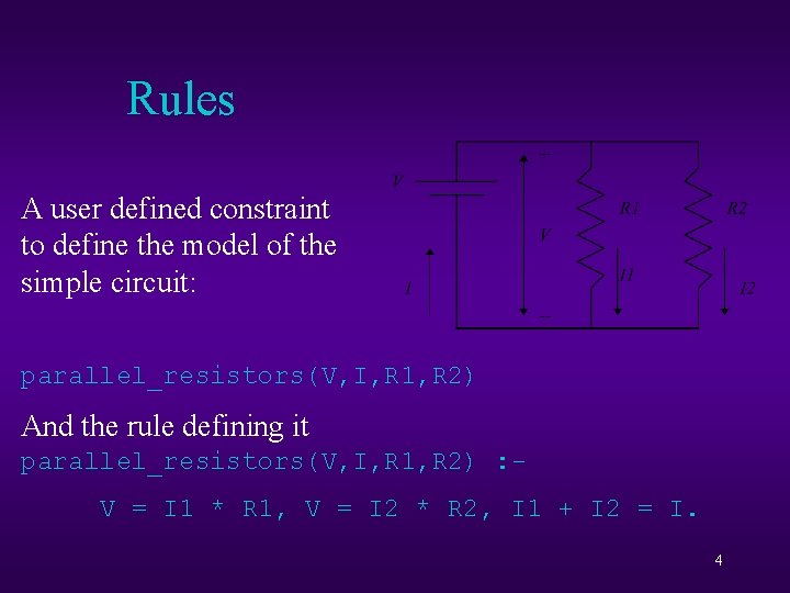
Rules A user defined constraint to define the model of the simple circuit: parallel_resistors(V, I, R 1, R 2) And the rule defining it parallel_resistors(V, I, R 1, R 2) : V = I 1 * R 1, V = I 2 * R 2, I 1 + I 2 = I. 4

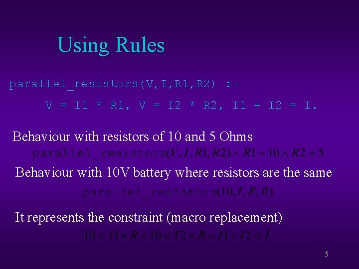
Using Rules parallel_resistors(V, I, R 1, R 2) : V = I 1 * R 1, V = I 2 * R 2, I 1 + I 2 = I. Behaviour with resistors of 10 and 5 Ohms Behaviour with 10 V battery where resistors are the same It represents the constraint (macro replacement) 5

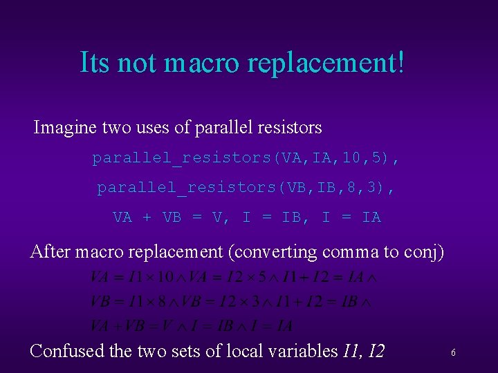
Its not macro replacement! Imagine two uses of parallel resistors parallel_resistors(VA, IA, 10, 5), parallel_resistors(VB, IB, 8, 3), VA + VB = V, I = IB, I = IA After macro replacement (converting comma to conj) Confused the two sets of local variables I 1, I 2 6

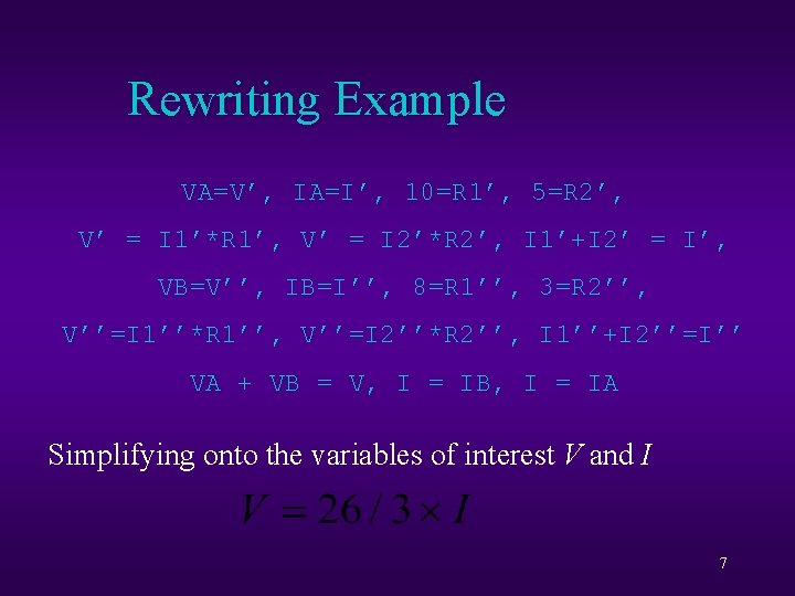
Rewriting Example parallel_resistors(VA, IA, 10, 5), VA=V’, IA=I’, 10=R 1’, 5=R 2’, V’ V’ ==parallel_resistors(VB, IB, 8, 3), I 1’*R 1’, V’ V’ == I 2’*R 2’, I 1’+I 2’ == I’, VA + VB IB=I’’, = V, I =8=R 1’’, IB, I =3=R 2’’, IA parallel_resistors(VB, IB, 8, 3), VB=V’’, V’’=I 1’’*R 1’’, VA + VB V’’=I 2’’*R 2’’, = V, rule I = IB, I I 1’’+I 2’’=I’’ = IA Rewrite the first literal with VA + VB = V, I = IB, I = IA parallel_resistors(V, I, R 1, R 2) : - Rewrite the. I 1 8 th*literal V = = I 2 *of. R 2, I 1 + I 2 = Simplifying onto. R 1, the Vvariables interest V and I I. Renaming: parallel_resistors(V’’, I’’, R 1’’, R 2’’) : parallel_resistors(V’, I’, R 1’, R 2’) : - 7 V’’=I 1’’*R 1’’, V’’=I 2’’*R 2’’, I 1’’+I 2’’=I’’. V’ = I 1’*R 1’, V’ = I 2’*R 2’, I 1’+I 2’ = I’.

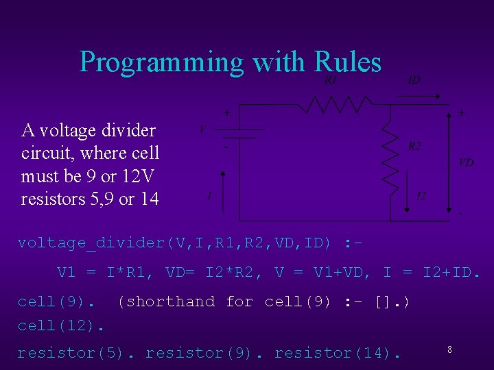
Programming with Rules A voltage divider circuit, where cell must be 9 or 12 V resistors 5, 9 or 14 voltage_divider(V, I, R 1, R 2, VD, ID) : V 1 = I*R 1, VD= I 2*R 2, V = V 1+VD, I = I 2+ID. cell(9). (shorthand for cell(9) : - []. ) cell(12). resistor(5). resistor(9). resistor(14). 8

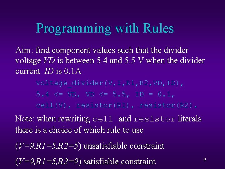
Programming with Rules Aim: find component values such that the divider voltage VD is between 5. 4 and 5. 5 V when the divider current ID is 0. 1 A voltage_divider(V, I, R 1, R 2, VD, ID), 5. 4 <= VD, VD <= 5. 5, ID = 0. 1, cell(V), resistor(R 1), resistor(R 2). Note: when rewriting cell and resistor literals there is a choice of which rule to use (V=9, R 1=5, R 2=5) unsatisfiable constraint (V=9, R 1=5, R 2=9) satisfiable constraint 9

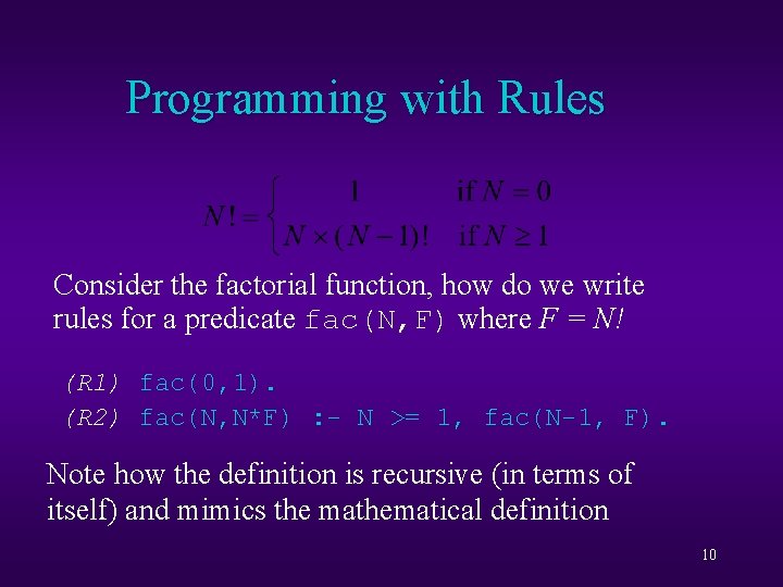
Programming with Rules Consider the factorial function, how do we write rules for a predicate fac(N, F) where F = N! (R 1) fac(0, 1). (R 2) fac(N, N*F) : - N >= 1, fac(N-1, F). Note how the definition is recursive (in terms of itself) and mimics the mathematical definition 10

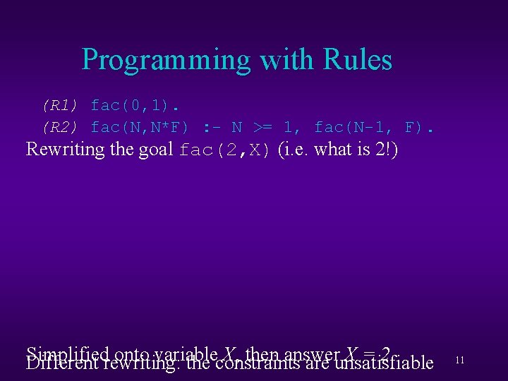
Programming with Rules (R 1) fac(0, 1). (R 2) fac(N, N*F) : - N >= 1, fac(N-1, F). Rewriting the goal fac(2, X) (i. e. what is 2!) Simplified onto variable X, then answer X=2 Different rewriting: the constraints are unsatisfiable 11

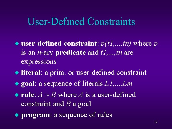
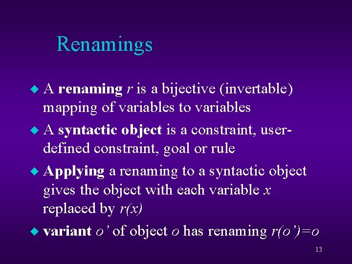
User-Defined Constraints user-defined constraint: p(t 1, . . . , tn) where p is an n-ary predicate and t 1, . . . , tn are expressions u literal: a prim. or user-defined constraint u goal: a sequence of literals L 1, . . . , Lm u rule: A : - B where A is a user-defined constraint and B a goal u program: a sequence of rules u 12

Renamings A renaming r is a bijective (invertable) mapping of variables to variables u A syntactic object is a constraint, userdefined constraint, goal or rule u Applying a renaming to a syntactic object gives the object with each variable x replaced by r(x) u variant o’ of object o has renaming r(o’)=o u 13

Rewriting User-Defined Cons. u goal G of the form (or empty m=0 []) u L 1, . . . , Li-1, Li+1, . . . , Lm Li is of the form p(t 1, . . . , tn) u R is of the form p(s 1, . . . , sn) : - B u r is a renaming s. t. vars in r(R) not in G u The rewriting of G at Li by R using renaming r is u u L 1, . . . , Li-1, t 1=r(s 1), . . . , tn=r(sn), r(B), Li+1, . . . , Lm 14

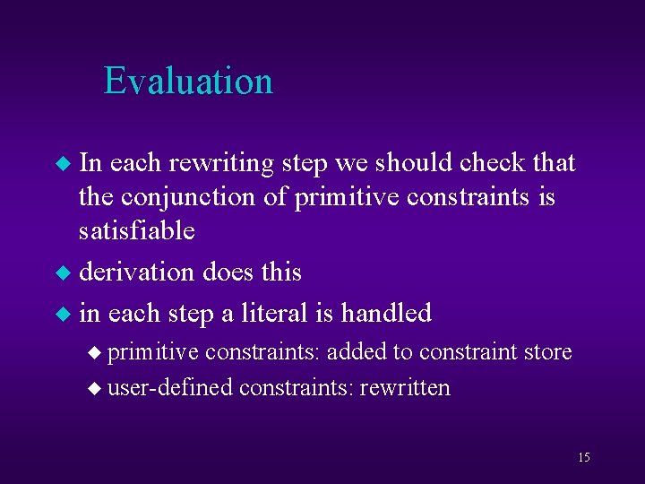
Evaluation In each rewriting step we should check that the conjunction of primitive constraints is satisfiable u derivation does this u in each step a literal is handled u u primitive constraints: added to constraint store u user-defined constraints: rewritten 15

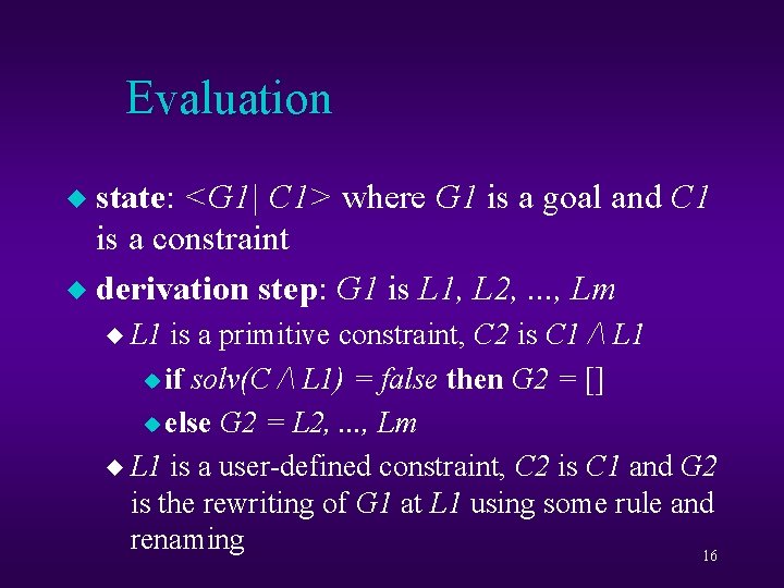
Evaluation state: <G 1| C 1> where G 1 is a goal and C 1 is a constraint u derivation step: G 1 is L 1, L 2, . . . , Lm u u L 1 is a primitive constraint, C 2 is C 1 / L 1 u if solv(C / L 1) = false then G 2 = [] u else G 2 = L 2, . . . , Lm u L 1 is a user-defined constraint, C 2 is C 1 and G 2 is the rewriting of G 1 at L 1 using some rule and renaming 16

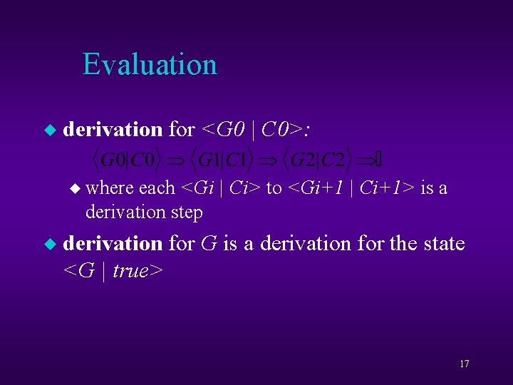
Evaluation u derivation for <G 0 | C 0>: u where each <Gi | Ci> to <Gi+1 | Ci+1> is a derivation step u derivation for G is a derivation for the state <G | true> 17

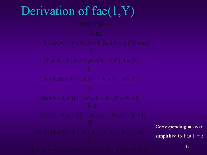
Derivation of fac(1, Y) Corresponding answer simplified to Y is Y = 1 18

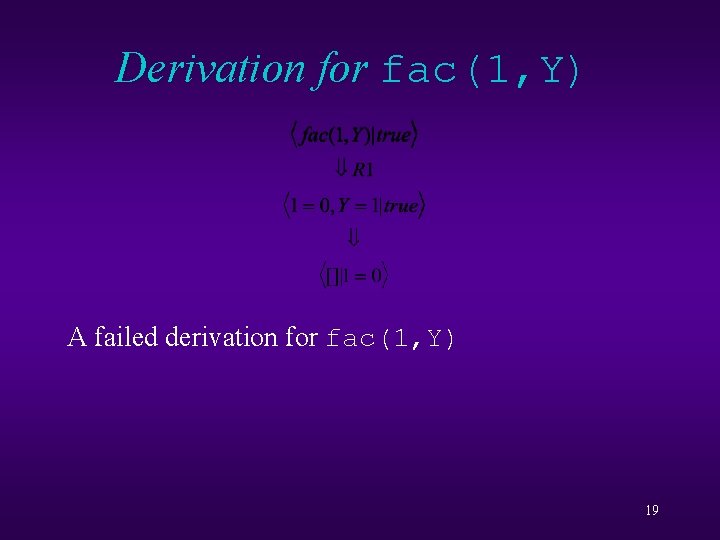
Derivation for fac(1, Y) A failed derivation for fac(1, Y) 19

Derivations For derivation beginning at <G 0 | C 0> u success state: <[] | C> where solv(C) != false u successful derivation: last state is success u answer: simpl(C, vars(<G 0 | C 0>)) u fail state: <[] | C> where solv(C) = false u failed derivation: last state is fail state u 20

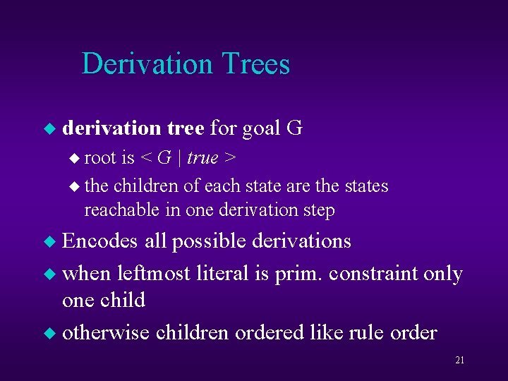
Derivation Trees u derivation tree for goal G u root is < G | true > u the children of each state are the states reachable in one derivation step Encodes all possible derivations u when leftmost literal is prim. constraint only one child u otherwise children ordered like rule order u 21

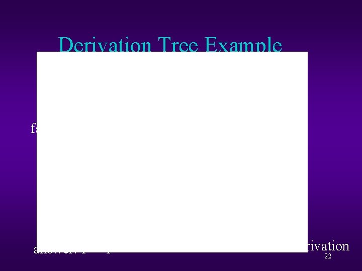
Derivation Tree Example failed derivation answer: Y = 1 failed derivation 22

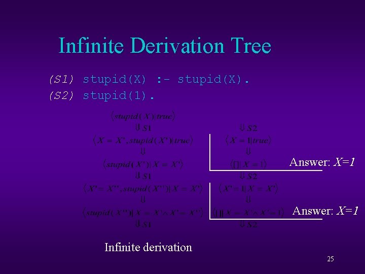
Derivation Trees The previous example shows three derivations, 2 failed and one successful u finitely failed: if a derivation tree is finite and all derivations are failed u next slide a finitely failed derivation tree u infinite derivation tree: some derivations are infinite u 23

Finitely Failed Example 24

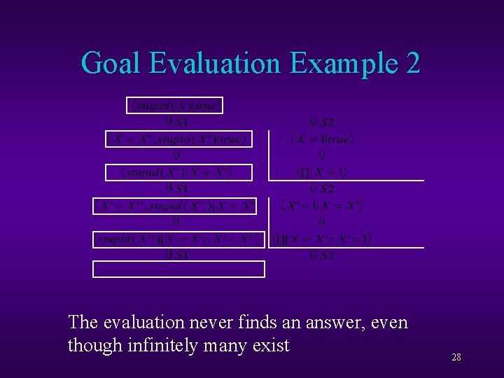
Infinite Derivation Tree (S 1) stupid(X) : - stupid(X). (S 2) stupid(1). Answer: X=1 Infinite derivation 25

Goal Evaluation of a goal performs an in-order depth-first search of the derivation tree u when a success state in encountered the system returns an answer u the user can ask for more answers in which case the search continues u execution halts when the users requests no more answers or the entire tree is explored u 26

Goal Evaluation Example Return answer: Y = 1 more? Return no 27 more

Goal Evaluation Example 2 The evaluation never finds an answer, even though infinitely many exist 28

Simplified Derivation Trees Derivation trees are very large u A simplified form which has the most useful information u u constraints in simplified form (variables in the initial goal and goal part of state) u uninteresting states removed 29

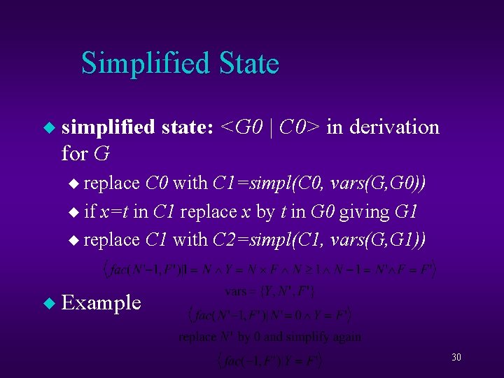
Simplified State u simplified state: <G 0 | C 0> in derivation for G u replace C 0 with C 1=simpl(C 0, vars(G, G 0)) u if x=t in C 1 replace x by t in G 0 giving G 1 u replace C 1 with C 2=simpl(C 1, vars(G, G 1)) u Example 30

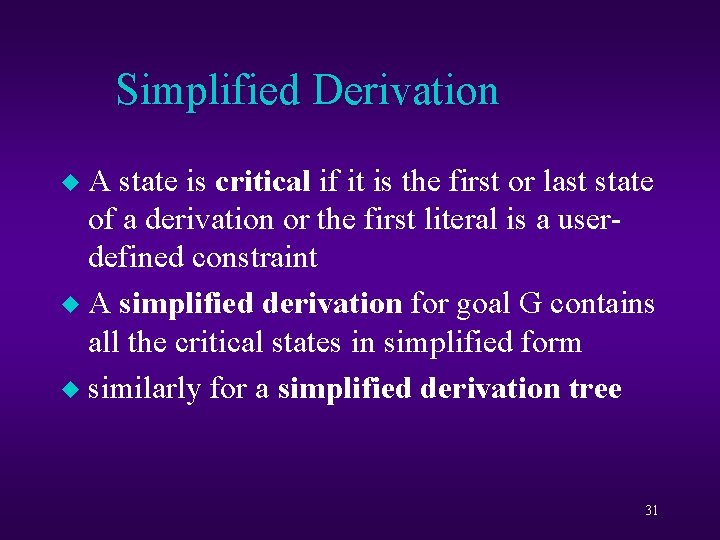
Simplified Derivation A state is critical if it is the first or last state of a derivation or the first literal is a userdefined constraint u A simplified derivation for goal G contains all the critical states in simplified form u similarly for a simplified derivation tree u 31

Example Simplified Tree Note: fail states are <[] | false> and success states contain answers 32

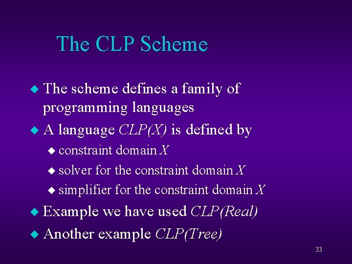
The CLP Scheme The scheme defines a family of programming languages u A language CLP(X) is defined by u u constraint domain X u solver for the constraint domain X u simplifier for the constraint domain X Example we have used CLP(Real) u Another example CLP(Tree) u 33

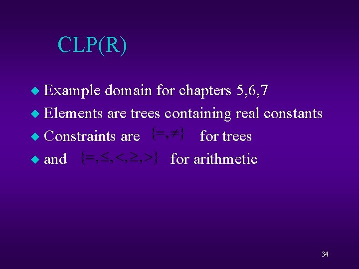
CLP(R) Example domain for chapters 5, 6, 7 u Elements are trees containing real constants u Constraints are for trees u and for arithmetic u 34

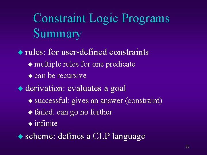
Constraint Logic Programs Summary u rules: for user-defined constraints u multiple rules for one predicate u can be recursive u derivation: evaluates a goal u successful: gives an answer (constraint) u failed: can go no further u infinite u scheme: defines a CLP language 35