Conditional Control Flow Constructs Sequential Control Flow Execution

Conditional Control Flow Constructs

Sequential Control Flow • Execution order follows the textual order • straight line flow • Many simple problems can not be solved only with such sequential flow • Here is an example • Problem: Computation of a maximum of two numbers

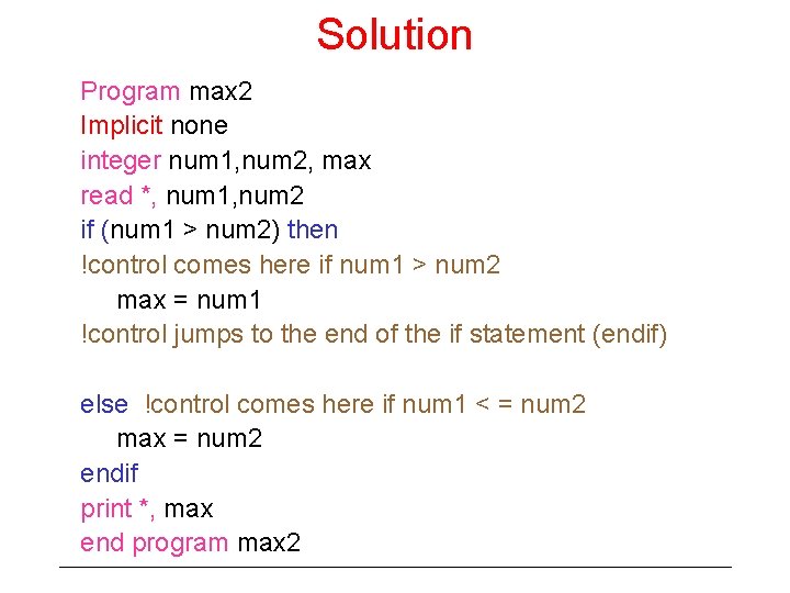
Solution Program max 2 Implicit none integer num 1, num 2, max read *, num 1, num 2 if (num 1 > num 2) then !control comes here if num 1 > num 2 max = num 1 !control jumps to the end of the if statement (endif) else !control comes here if num 1 < = num 2 max = num 2 endif print *, max end program max 2

Another Problem • Input two numbers • Compute the quotient and remainder of the bigger number divided by the smaller number • The numbers are input in unknown order

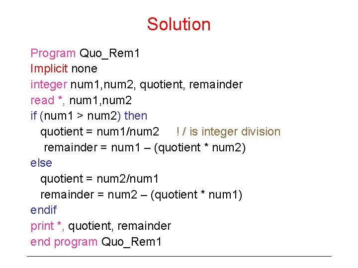
Solution Program Quo_Rem 1 Implicit none integer num 1, num 2, quotient, remainder read *, num 1, num 2 if (num 1 > num 2) then quotient = num 1/num 2 ! / is integer division remainder = num 1 – (quotient * num 2) else quotient = num 2/num 1 remainder = num 2 – (quotient * num 1) endif print *, quotient, remainder end program Quo_Rem 1

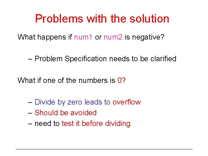
Problems with the solution What happens if num 1 or num 2 is negative? – Problem Specification needs to be clarified What if one of the numbers is 0? – Divide by zero leads to overflow – Should be avoided – need to test it before dividing

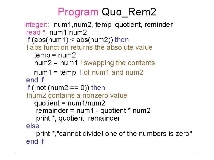
Program Quo_Rem 2 integer: : num 1, num 2, temp, quotient, reminder read *, num 1, num 2 if (abs(num 1) < abs(num 2)) then ! abs function returns the absolute value temp = num 2 = num 1 ! swapping the contents num 1 = temp ! of num 1 and num 2 end if if (. not. (num 2 == 0)) then !num 2 contains a nonzero value quotient = num 1/num 2 remainder = num 1 - quotient * num 2 print *, quotient, remainder else print *, "cannot divide! one of the numbers is zero" end if

The program Quo_Rem 2 • The body of if-then-else is simpler • The else clause is missing • Complex conditions can appear in the if-condition • Successive if-statements allowed

Another Problem • %Nesting of ifs Problem: Compute Maximum of three numbers Solution: ?

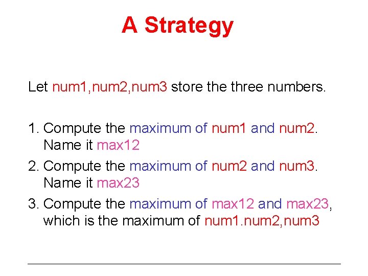
A Strategy Let num 1, num 2, num 3 store three numbers. 1. Compute the maximum of num 1 and num 2. Name it max 12 2. Compute the maximum of num 2 and num 3. Name it max 23 3. Compute the maximum of max 12 and max 23, which is the maximum of num 1. num 2, num 3

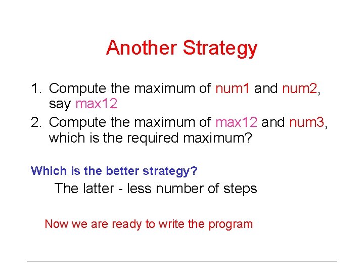
Another Strategy 1. Compute the maximum of num 1 and num 2, say max 12 2. Compute the maximum of max 12 and num 3, which is the required maximum? Which is the better strategy? The latter - less number of steps Now we are ready to write the program

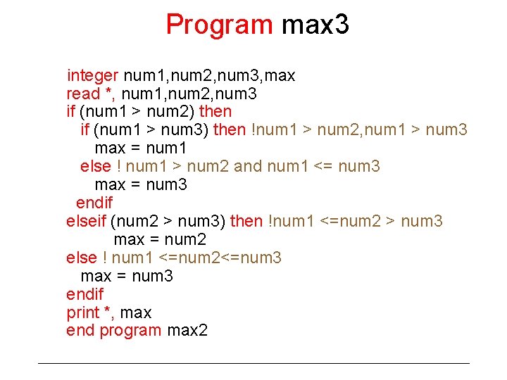
Program max 3 integer num 1, num 2, num 3, max read *, num 1, num 2, num 3 if (num 1 > num 2) then if (num 1 > num 3) then !num 1 > num 2, num 1 > num 3 max = num 1 else ! num 1 > num 2 and num 1 <= num 3 max = num 3 endif elseif (num 2 > num 3) then !num 1 <=num 2 > num 3 max = num 2 else ! num 1 <=num 2<=num 3 max = num 3 endif print *, max end program max 2

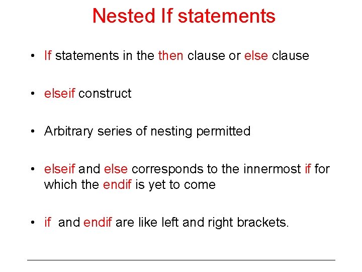
Nested If statements • If statements in then clause or else clause • elseif construct • Arbitrary series of nesting permitted • elseif and else corresponds to the innermost if for which the endif is yet to come • if and endif are like left and right brackets.

Further Observations • else clause can be missing • endif can be dropped if there is only one statement • long series of ifs can be confusing (at most 20 levels allowed) • indentation improves readability • use indentation and comments

If conditions • Control flow branches in conditional statements • Branching decided by evaluating the conditions • conditions are expressions of a new type called LOGICAL • Examples: (x > 0), (z == 1), . NOT. (num == 2) • All these involve relational operators: >, == • Relational operators are defined over many data types to compare values

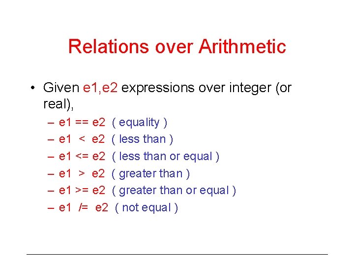
Relations over Arithmetic • Given e 1, e 2 expressions over integer (or real), – – – e 1 == e 2 ( equality ) e 1 < e 2 ( less than ) e 1 <= e 2 ( less than or equal ) e 1 > e 2 ( greater than ) e 1 >= e 2 ( greater than or equal ) e 1 /= e 2 ( not equal )

LOGICAL VARIABLES • Fortran 90 has a built in LOGICAL DATA TYPE • Expressions involving relational operators are of type LOGICAL • Variables can be declared to have type LOGICAL • Declarations: LOGICAL : : found, goodness • Logical variables assume just two values –. TRUE. , . FALSE. • They can be used in if conditions, eg. – if (found) then stop – if (goodness) then x = 0

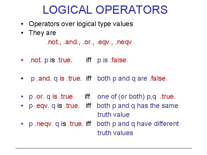
LOGICAL OPERATORS • Operators over logical type values • They are. not. , . and. , . or. , . eqv. , . neqv. • . not. p is. true. • iff p is. false. p. and. q is. true. iff both p and q are. false. • p. or. q is. true. iff one of (or both) p, q. true. • p. eqv. q is. true. iff both p and q has the same truth value • p. neqv. q is. true. iff both p and q have different truth values

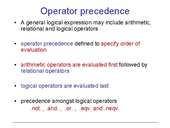
Operator precedence • A general logical expression may include arithmetic, relational and logical operators • operator precedence defined to specify order of evaluation • arithmetic operators are evaluated first followed by relational operators • logical operators are evaluated last • precedence amongst logical operators. not. , . and. , . or. , . eqv. and. neqv.

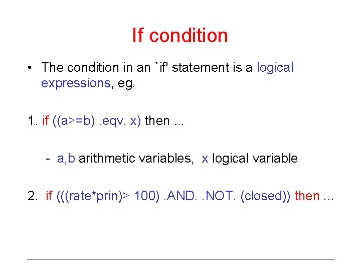
If condition • The condition in an `if' statement is a logical expressions, eg. 1. if ((a>=b). eqv. x) then. . . - a, b arithmetic variables, x logical variable 2. if (((rate*prin)> 100). AND. . NOT. (closed)) then. . .

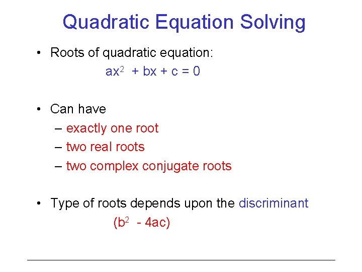
Quadratic Equation Solving • Roots of quadratic equation: ax 2 + bx + c = 0 • Can have – exactly one root – two real roots – two complex conjugate roots • Type of roots depends upon the discriminant (b 2 - 4 ac)

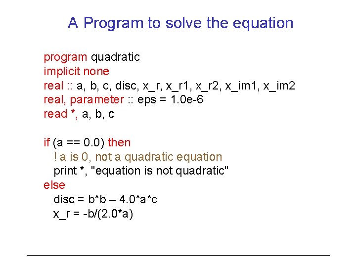
A Program to solve the equation program quadratic implicit none real : : a, b, c, disc, x_r 1, x_r 2, x_im 1, x_im 2 real, parameter : : eps = 1. 0 e-6 read *, a, b, c if (a == 0. 0) then ! a is 0, not a quadratic equation print *, "equation is not quadratic" else disc = b*b – 4. 0*a*c x_r = -b/(2. 0*a)

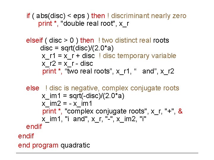
if ( abs(disc) < eps ) then ! discriminant nearly zero print *, "double real root", x_r elseif ( disc > 0 ) then ! two distinct real roots disc = sqrt(disc)/(2. 0*a) x_r 1 = x_r + disc ! disc temporary variable x_r 2 = x_r - disc print *, “two real roots”, x_r 1, “ and”, x_r 2 else ! disc is negative, complex conjugate roots x_im 1 = sqrt(-disc)/(2. 0*a) x_im 2 = - x_im 1 print *, "complex conjugate roots", x_r, "+", & x_im 1, "i and", x_r, "-", x_im 2, "i" endif end program quadratic

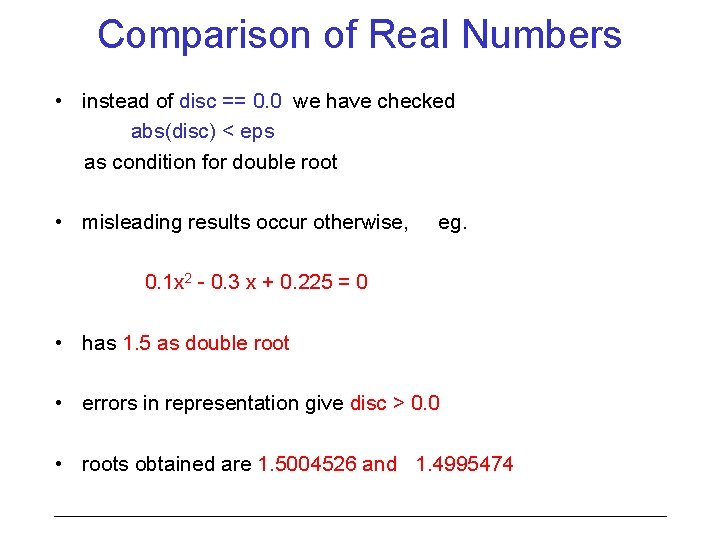
Comparison of Real Numbers • instead of disc == 0. 0 we have checked abs(disc) < eps as condition for double root • misleading results occur otherwise, eg. 0. 1 x 2 - 0. 3 x + 0. 225 = 0 • has 1. 5 as double root • errors in representation give disc > 0. 0 • roots obtained are 1. 5004526 and 1. 4995474

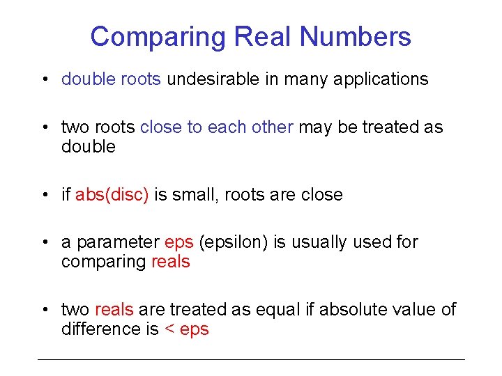
Comparing Real Numbers • double roots undesirable in many applications • two roots close to each other may be treated as double • if abs(disc) is small, roots are close • a parameter eps (epsilon) is usually used for comparing reals • two reals are treated as equal if absolute value of difference is < eps

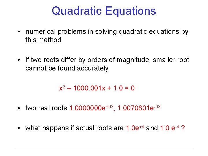
Quadratic Equations • numerical problems in solving quadratic equations by this method • if two roots differ by orders of magnitude, smaller root cannot be found accurately x 2 – 1000. 001 x + 1. 0 = 0 • two real roots 1. 0000000 e+03, 1. 0070801 e-03 • what happens if actual roots are 1. 0 e+4 and 1. 0 e-4 ?

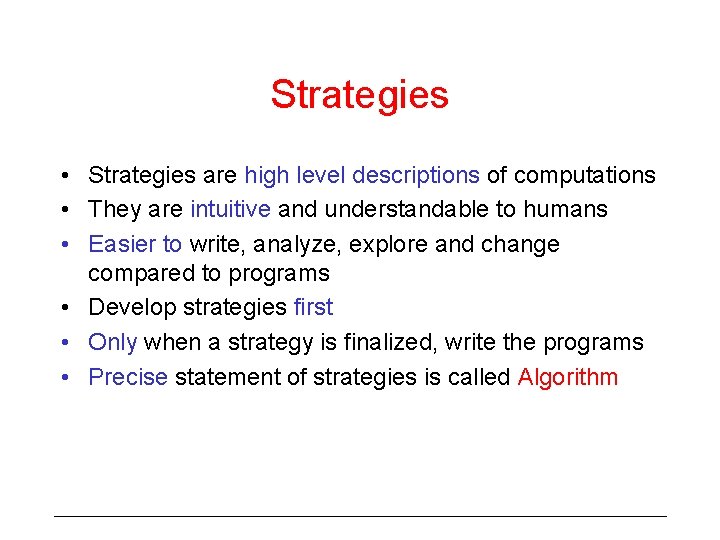
Strategies • Strategies are high level descriptions of computations • They are intuitive and understandable to humans • Easier to write, analyze, explore and change compared to programs • Develop strategies first • Only when a strategy is finalized, write the programs • Precise statement of strategies is called Algorithm

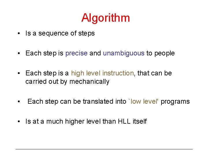
Algorithm • Is a sequence of steps • Each step is precise and unambiguous to people • Each step is a high level instruction, that can be carried out by mechanically • Each step can be translated into `low level' programs • Is at a much higher level than HLL itself

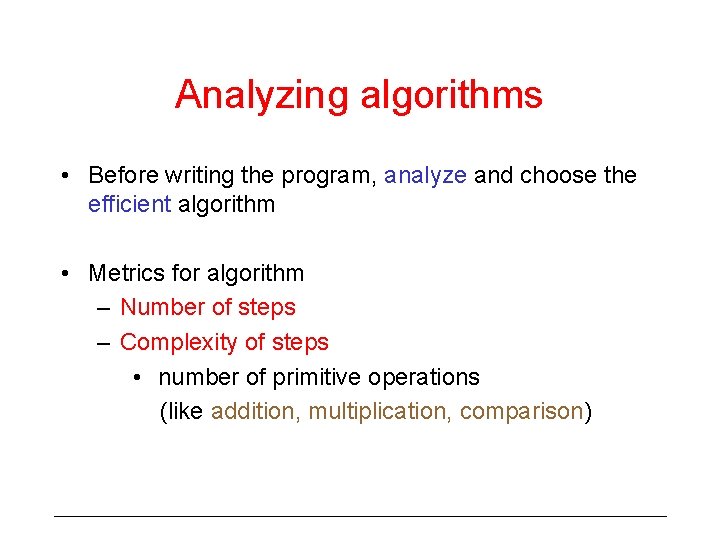
Analyzing algorithms • Before writing the program, analyze and choose the efficient algorithm • Metrics for algorithm – Number of steps – Complexity of steps • number of primitive operations (like addition, multiplication, comparison)