CMSC 28100 Lecture 7 Asymptotics Polynomial Time Time

CMSC 28100 – Lecture 7 Asymptotics, Polynomial Time

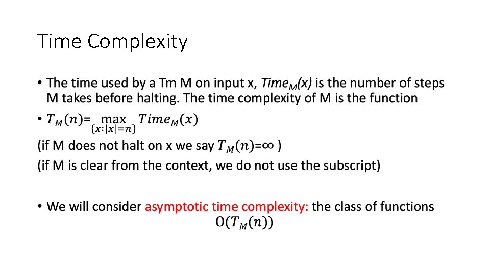
Time Complexity •

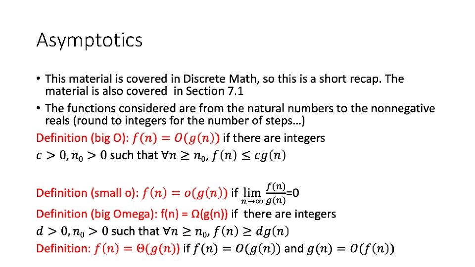
Asymptotics •

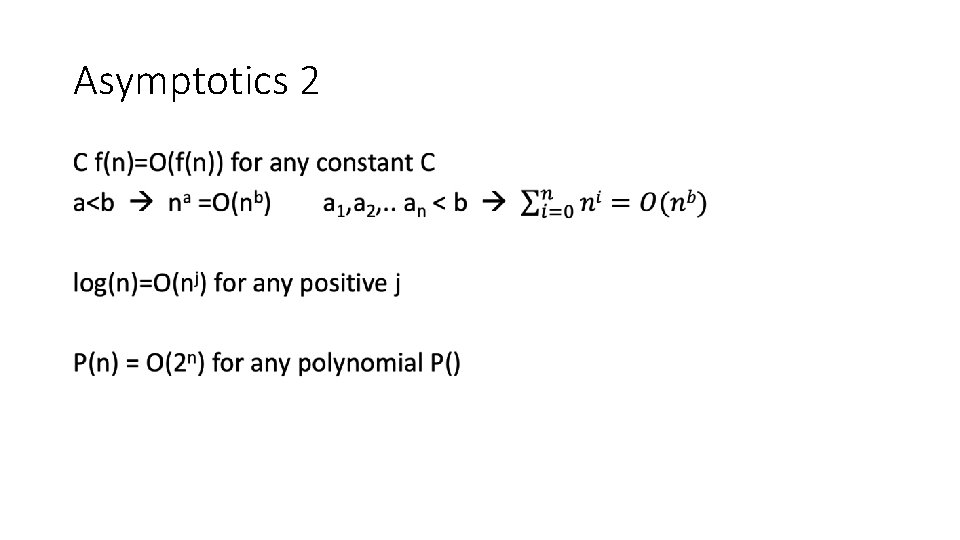
Asymptotics 2 •

Polynomial Time • P=Polynomial Time (Time. M(n) is a polynomial in n) • More precisely, let f(n) be a nondecreasing function. • Definition: TIME(f(n)) is the class of languages decidable by Turing machines that use O(f(n)) moves.

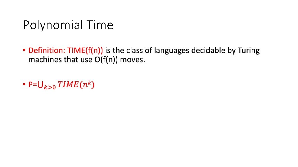
Polynomial Time •

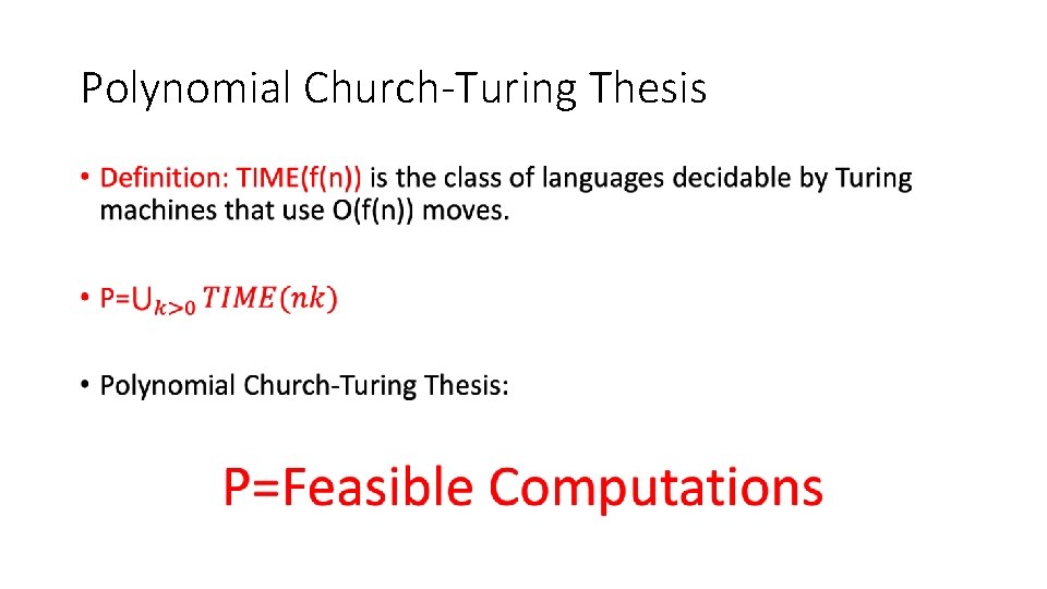
Polynomial Church-Turing Thesis •

Polynomial Time = Feasible • Justification for thesis: (See also Sipser 7. 1, Kleinberg-Tardos: Algorithm Design Chapter 2. ) 1. P is a nice class – closed under subroutines.

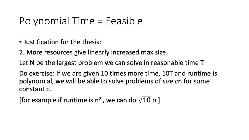
Polynomial Time = Feasible • Justification for thesis: (See also Sipser 7. 1, Kleinberg-Tardos: Algorithm Design Chapter 2. ) 1. P is a nice class – closed under subroutines. if g(x) and h(x) polynomial time computable, so is g(h(x)) 2. More resources give linearly increased max size.

Polynomial Time = Feasible •

Polynomial Time = Feasible • Justification for thesis: 1. P is a nice class – closed under subroutines. if g(x) and h(x) polynomial time computable, so is g(h(x)) 2. More resources give linearly increased max size. In contrast exponential time (2 n) has neither of theses nice properties.

Polynomial Time = Feasible • Justification for thesis: 1. P is a nice class – closed under subroutines. if g(x) and h(x) polynomial time computable, so is g(h(x)) 2. More resources give linearly increased max size. In contrast exponential time (2 n) has neither of theses nice properties. 3. Robust notion under different models of computation

Polynomial Time = Feasible Robust notion under different models of computation Theorem: For fixed k, k-tape Tms running in time t can be simulated by a 1 -tape Tm running in time O(t 2). [Challenging exercise: k tape machines can be simulated by 2 -tape machines in time t log t]

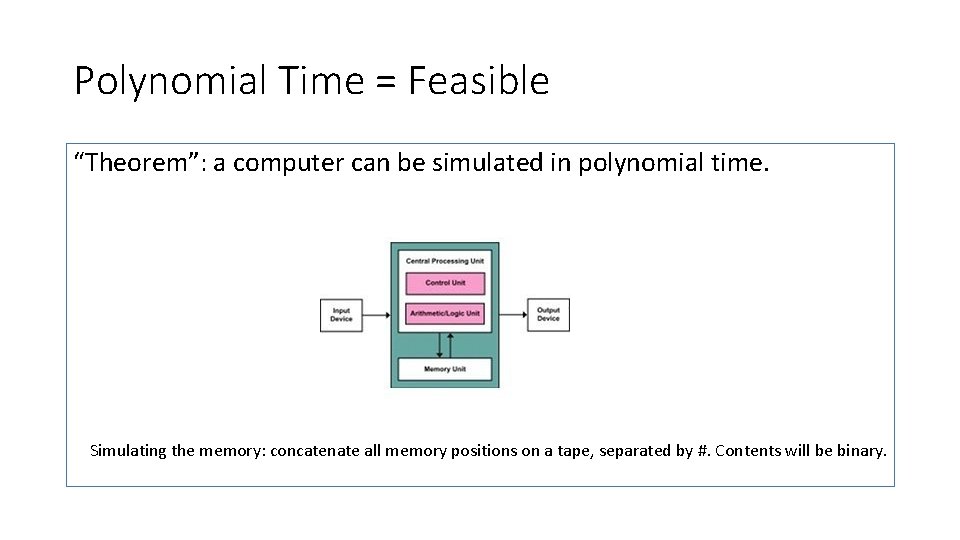
Polynomial Time = Feasible Robust notion under different models of computation Theorem: For fixed k, k-tape Tms running in time t can be simulated by a 1 -tape Tm running in time O(t 2). “Theorem”: a computer can be simulated in polynomial time.

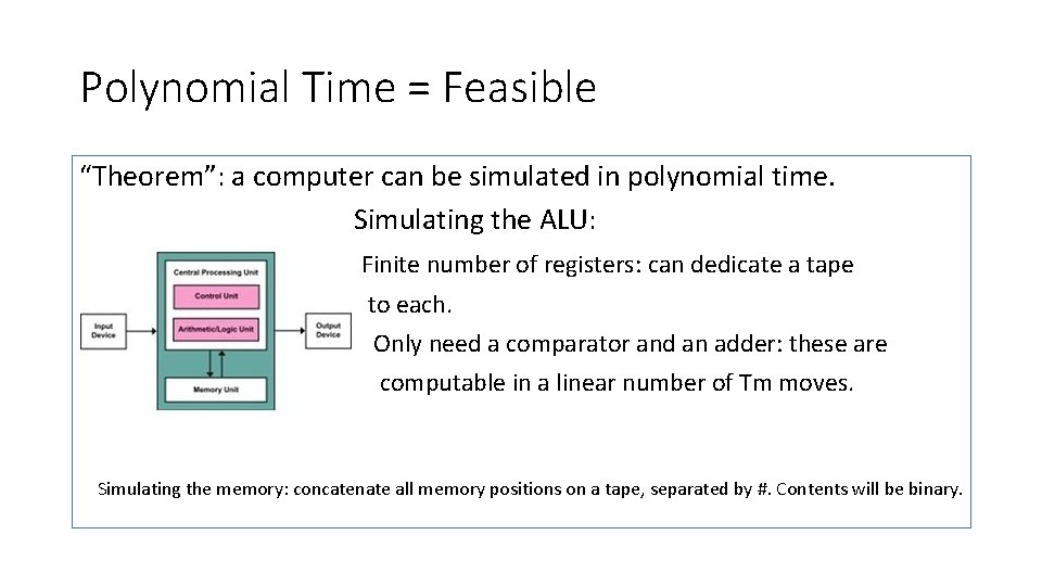
Polynomial Time = Feasible “Theorem”: a computer can be simulated in polynomial time. Simulating the memory: concatenate all memory positions on a tape, separated by #. Contents will be binary.

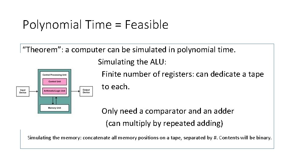
Polynomial Time = Feasible “Theorem”: a computer can be simulated in polynomial time. Simulating the ALU: Finite number of registers: can dedicate a tape to each. Only need a comparator and an adder (can multiply by repeated adding) Simulating the memory: concatenate all memory positions on a tape, separated by #. Contents will be binary.

Polynomial Time = Feasible “Theorem”: a computer can be simulated in polynomial time. Simulating the ALU: Finite number of registers: can dedicate a tape to each. Only need a comparator and an adder: these are computable in a linear number of Tm moves. Simulating the memory: concatenate all memory positions on a tape, separated by #. Contents will be binary.

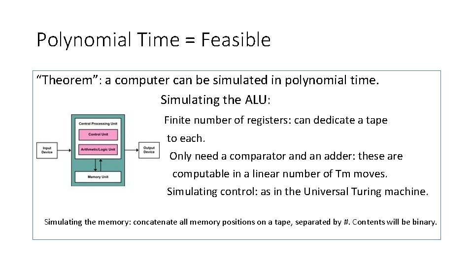
Polynomial Time = Feasible “Theorem”: a computer can be simulated in polynomial time. Simulating the ALU: Finite number of registers: can dedicate a tape to each. Only need a comparator and an adder: these are computable in a linear number of Tm moves. Simulating control: as in the Universal Turing machine. Simulating the memory: concatenate all memory positions on a tape, separated by #. Contents will be binary.

Polynomial Time = Feasible ? • Is P too big? n 50 does not seem very feasible…. • No other class a good candidate • Many interesting algorithms have low degree polynomial algorithms. In several cases the initial algorithm was a higher degree polynomial. .

NP

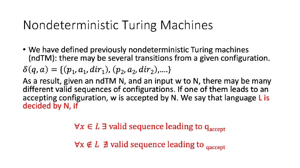
Nondeterministic Turing Machines •

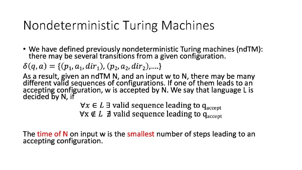
Nondeterministic Turing Machines •

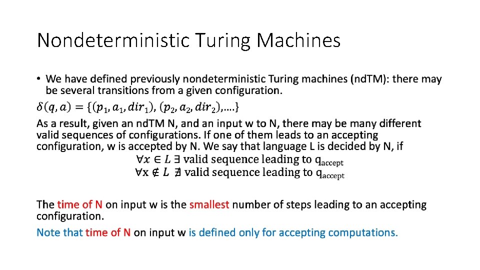
Nondeterministic Turing Machines •

Nondeterministic Turing Machines •

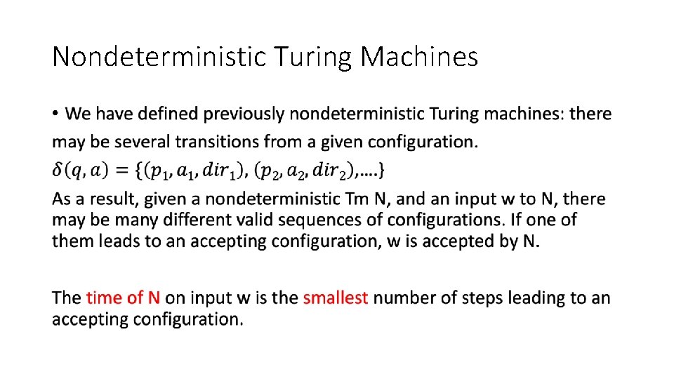
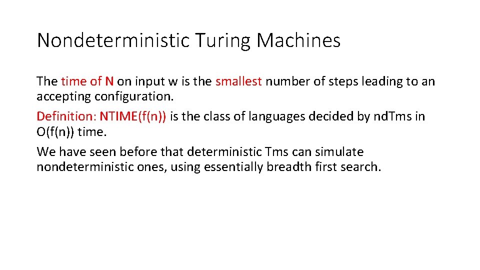
Nondeterministic Turing Machines The time of N on input w is the smallest number of steps leading to an accepting configuration. Definition: NTIME(f(n)) is the class of languages decided by nd. Tms in O(f(n)) time. We have seen before that deterministic Tms can simulate nondeterministic ones, using essentially breadth first search.

Nondeterministic Turing Machines The time of N on input w is the smallest number of steps leading to an accepting configuration. Definition: NTIME(f(n)) is the class of languages decided by nd. Tms in O(f(n)) time. We have seen before that deterministic Tms can simulate nondeterministic ones, using essentially breadth first search. However, this simulation requires 2 O(f(n)) time!

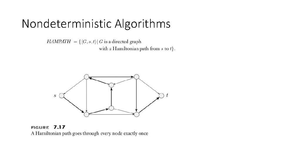
Nondeterministic Algorithms

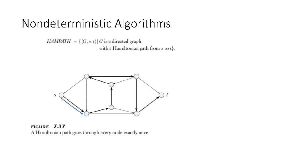
Nondeterministic Algorithms

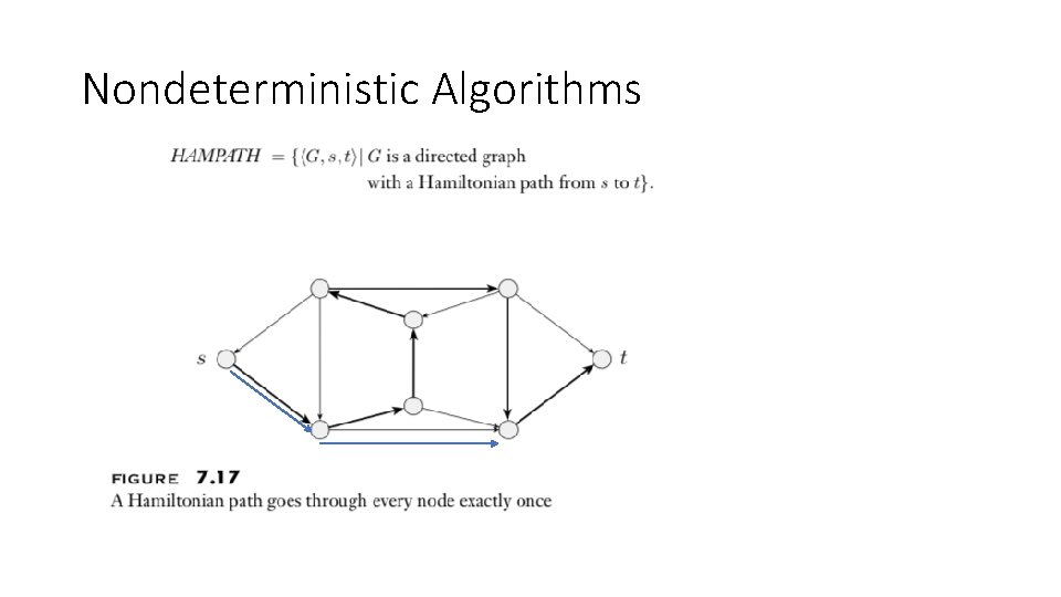
Nondeterministic Algorithms

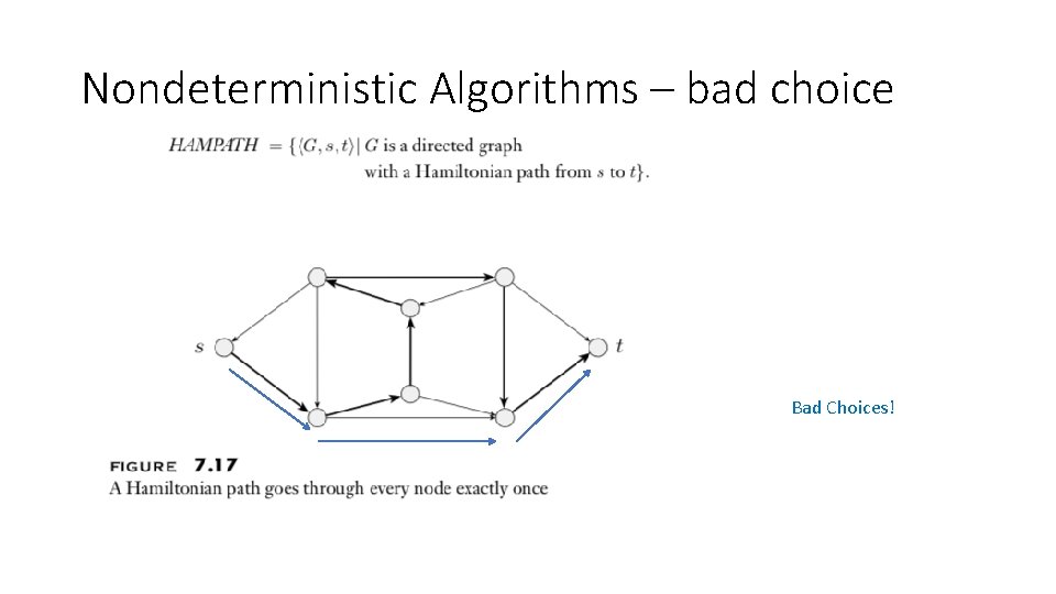
Nondeterministic Algorithms – bad choice Bad Choices!

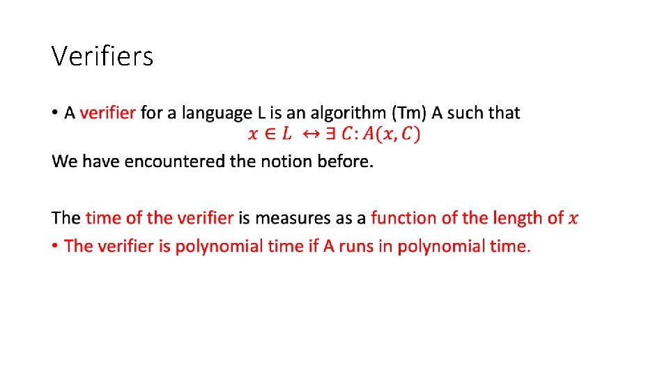
Verifiers •

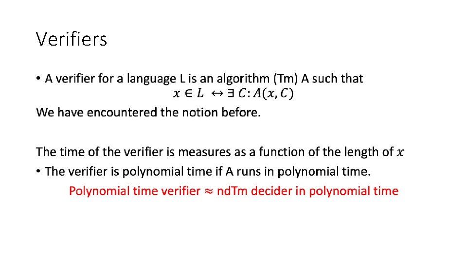
Verifiers •

Verifiers • Intuition: nd. TMs can guess a solution, then check it. (the checking is deterministic)

Verifiers • Intuition: nd. TMs can guess a solution, then check it. (the checking is deterministic) • Alternatively: the computation becomes deterministic once given the decision at each nondeterministic move.

Verifiers • Intuition: nd. TMs can guess a solution, then check it. (the checking is deterministic) • Alternatively: the computation becomes deterministic once given the decision at each nondeterministic move. • Yet another way to state it: nondeterministic machines can make all nondeterministic moves at the beginning of the computation

P, NP P=NP ?