CHEME 7130 Process Modeling Lecture 4 1 Lecutre

CHEM-E 7130 Process Modeling Lecture 4 1

Lecutre 4 outline • Which models lead to partial differential equations? • Coupled and uncoupled physical models • Some solution methods: – finite differences – polynomial approximations – finite volume 2

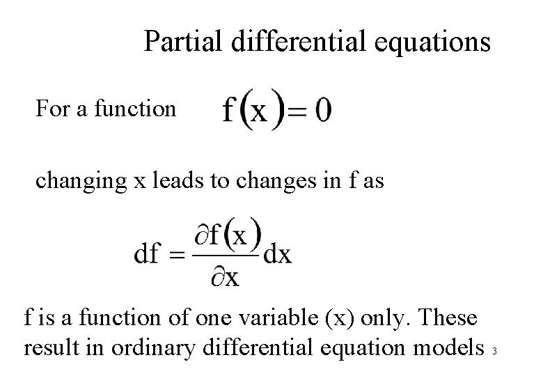
Partial differential equations For a function changing x leads to changes in f as f is a function of one variable (x) only. These result in ordinary differential equation models 3

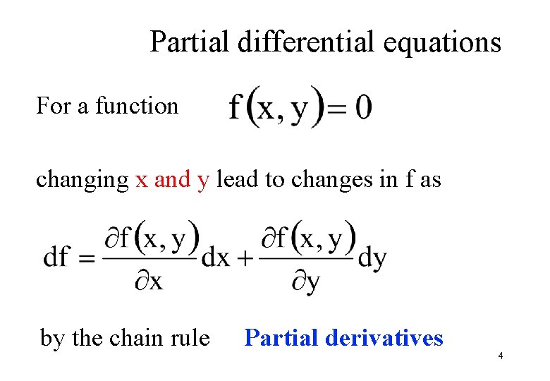
Partial differential equations For a function changing x and y lead to changes in f as by the chain rule Partial derivatives 4

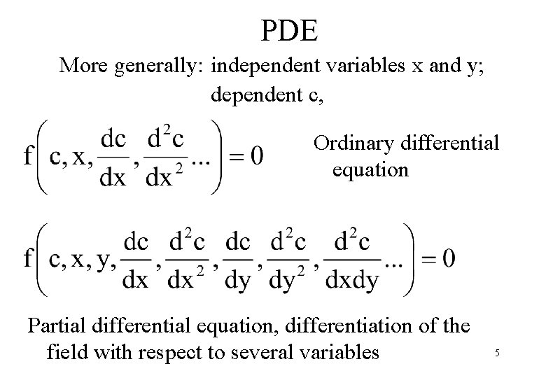
PDE More generally: independent variables x and y; dependent c, Ordinary differential equation Partial differential equation, differentiation of the field with respect to several variables 5

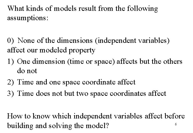
What kinds of models result from the following assumptions: 0) None of the dimensions (independent variables) affect our modeled property 1) One dimension (time or space) affects but the others do not 2) Time and one space coordinate affect 3) Time does not but two space coordinates affect How to know which independent variables affect before 6 building and solving the model?

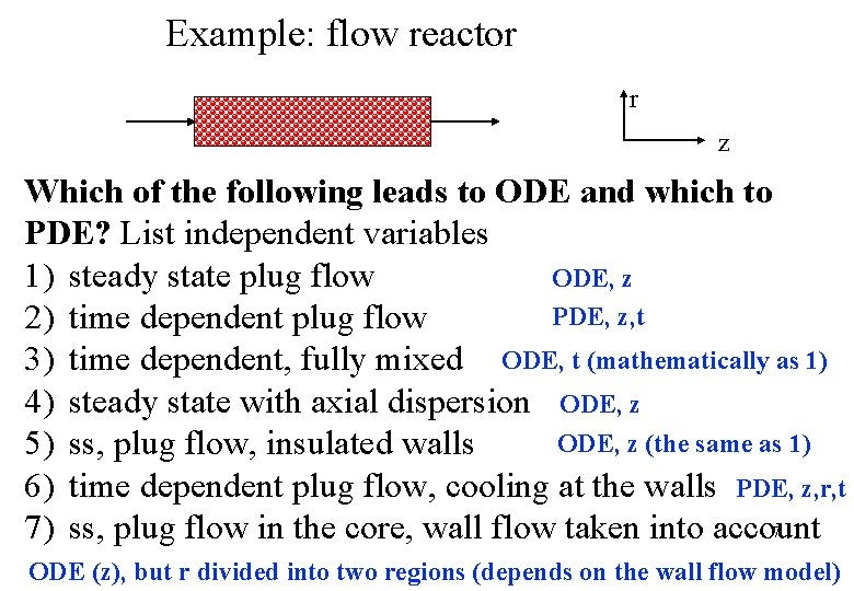
Example: flow reactor r z Which of the following leads to ODE and which to PDE? List independent variables 1) steady state plug flow ODE, z PDE, z, t 2) time dependent plug flow 3) time dependent, fully mixed ODE, t (mathematically as 1) 4) steady state with axial dispersion ODE, z (the same as 1) 5) ss, plug flow, insulated walls 6) time dependent plug flow, cooling at the walls PDE, z, r, t 7 7) ss, plug flow in the core, wall flow taken into account ODE (z), but r divided into two regions (depends on the wall flow model)

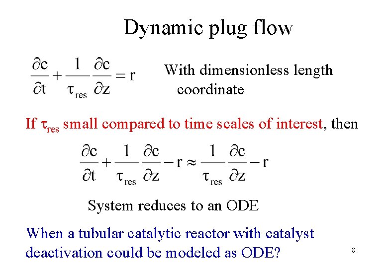
Dynamic plug flow With dimensionless length coordinate If res small compared to time scales of interest, then System reduces to an ODE When a tubular catalytic reactor with catalyst deactivation could be modeled as ODE? 8

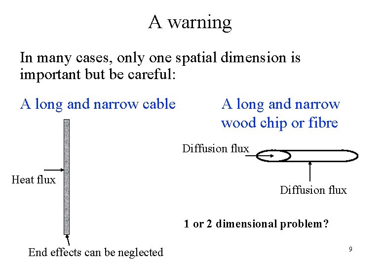
A warning In many cases, only one spatial dimension is important but be careful: A long and narrow cable A long and narrow wood chip or fibre Diffusion flux Heat flux Diffusion flux 1 or 2 dimensional problem? End effects can be neglected 9

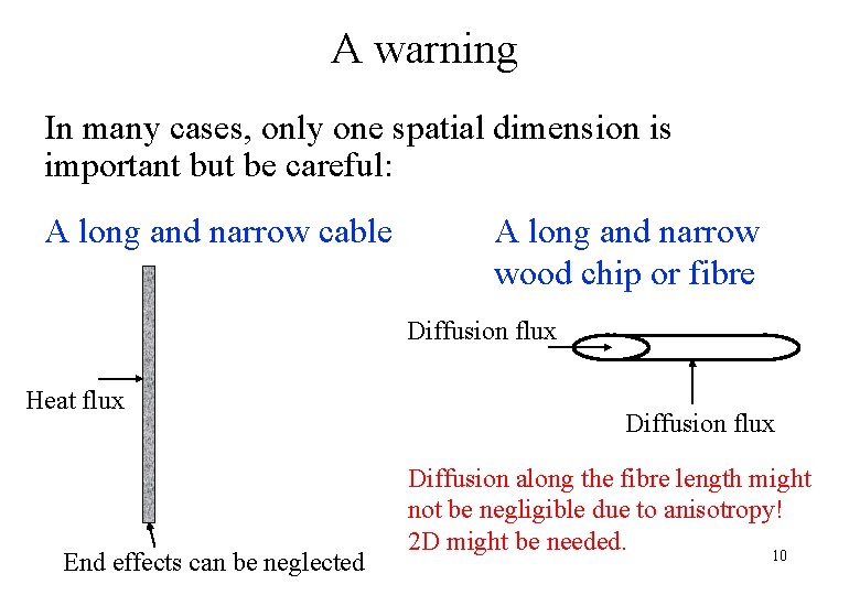
A warning In many cases, only one spatial dimension is important but be careful: A long and narrow cable A long and narrow wood chip or fibre Diffusion flux Heat flux End effects can be neglected Diffusion flux Diffusion along the fibre length might not be negligible due to anisotropy! 2 D might be needed. 10

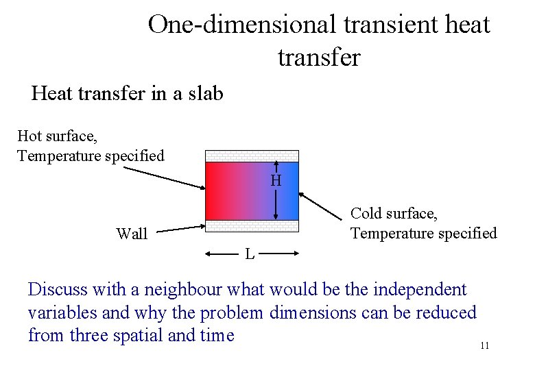
One-dimensional transient heat transfer Heat transfer in a slab Hot surface, Temperature specified H Cold surface, Temperature specified Wall L Discuss with a neighbour what would be the independent variables and why the problem dimensions can be reduced from three spatial and time 11

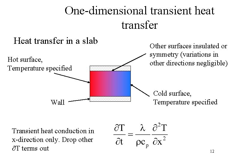
One-dimensional transient heat transfer Heat transfer in a slab Hot surface, Temperature specified Wall Transient heat conduction in x-direction only. Drop other T terms out Other surfaces insulated or symmetry (variations in other directions negligible) Cold surface, Temperature specified 12

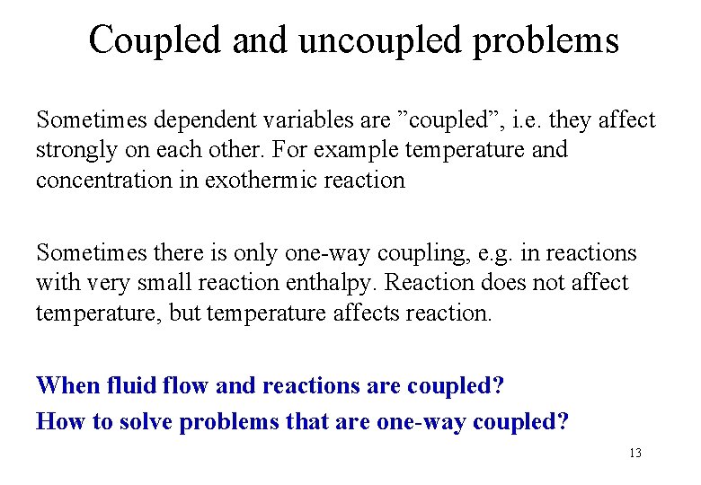
Coupled and uncoupled problems Sometimes dependent variables are ”coupled”, i. e. they affect strongly on each other. For example temperature and concentration in exothermic reaction Sometimes there is only one-way coupling, e. g. in reactions with very small reaction enthalpy. Reaction does not affect temperature, but temperature affects reaction. When fluid flow and reactions are coupled? How to solve problems that are one-way coupled? 13

Some solution methods Usually partial differential equations are discretized in some way to transform them to a set of ordinary differential equations Similar methods can be used to solve ordinary differential equations (transform them into a set of algebraic equations) There are numerous methods for this. 14

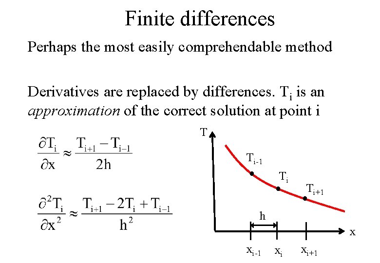
Finite differences Perhaps the most easily comprehendable method Derivatives are replaced by differences. Ti is an approximation of the correct solution at point i T Ti-1 Ti Ti+1 h x xi-1 xi xi+1

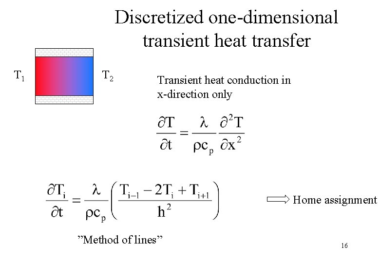
Discretized one-dimensional transient heat transfer T 1 T 2 Transient heat conduction in x-direction only Home assignment ”Method of lines” 16

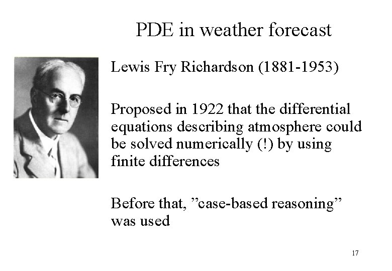
PDE in weather forecast Lewis Fry Richardson (1881 -1953) Proposed in 1922 that the differential equations describing atmosphere could be solved numerically (!) by using finite differences Before that, ”case-based reasoning” was used 17

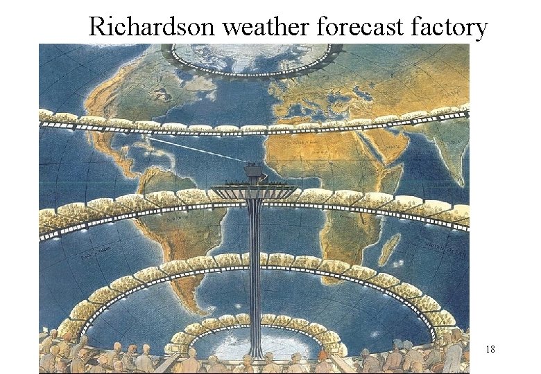
Richardson weather forecast factory 18

Richardson weather forecast factory Richardson estimated that 64 000 people would be needed to keep pace with the atmosphere Already in 2008, computer capacity in European weather forecast was ~1010 times faster than the Richardson factory, corresponding to ~1015 people doing hand calculations Also numerical methods have evolved considerably 19

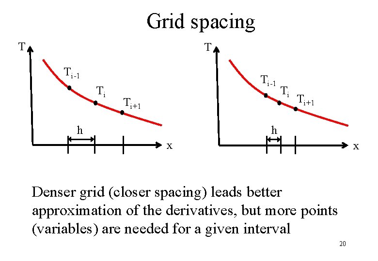
Grid spacing T T Ti-1 Ti+1 Ti Ti+1 h h x x Denser grid (closer spacing) leads better approximation of the derivatives, but more points (variables) are needed for a given interval 20

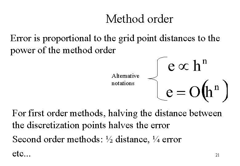
Method order Error is proportional to the grid point distances to the power of the method order Alternative notations For first order methods, halving the distance between the discretization points halves the error Second order methods: ½ distance, ¼ error etc. . . 21

Method order • Usually low order methods are inaccurate (numerical diffusion) • High order method are often less stable or are susceptible to oscillations • High order does not necessarily mean more accurate 22

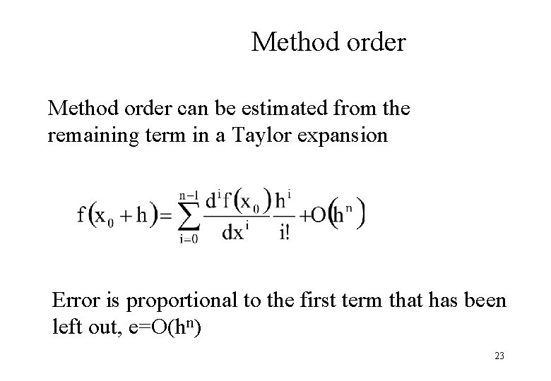
Method order can be estimated from the remaining term in a Taylor expansion Error is proportional to the first term that has been left out, e=O(hn) 23

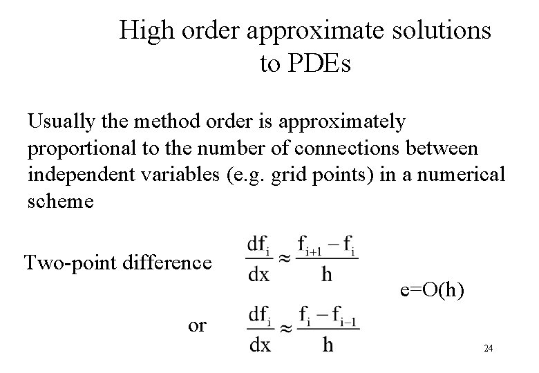
High order approximate solutions to PDEs Usually the method order is approximately proportional to the number of connections between independent variables (e. g. grid points) in a numerical scheme Two-point difference e=O(h) or 24

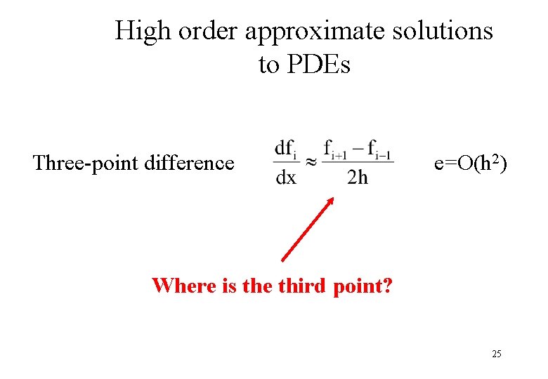
High order approximate solutions to PDEs Three-point difference e=O(h 2) Where is the third point? 25

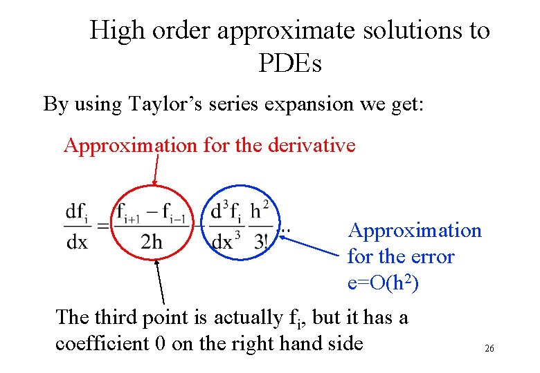
High order approximate solutions to PDEs By using Taylor’s series expansion we get: Approximation for the derivative Approximation for the error e=O(h 2) The third point is actually fi, but it has a coefficient 0 on the right hand side 26

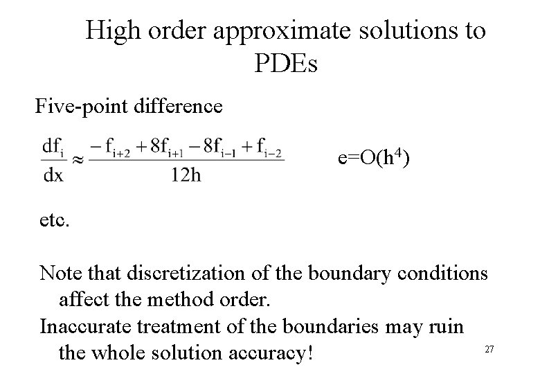
High order approximate solutions to PDEs Five-point difference e=O(h 4) etc. Note that discretization of the boundary conditions affect the method order. Inaccurate treatment of the boundaries may ruin 27 the whole solution accuracy!

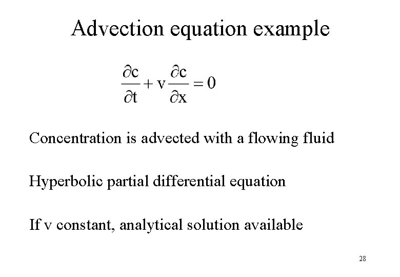
Advection equation example Concentration is advected with a flowing fluid Hyperbolic partial differential equation If v constant, analytical solution available 28

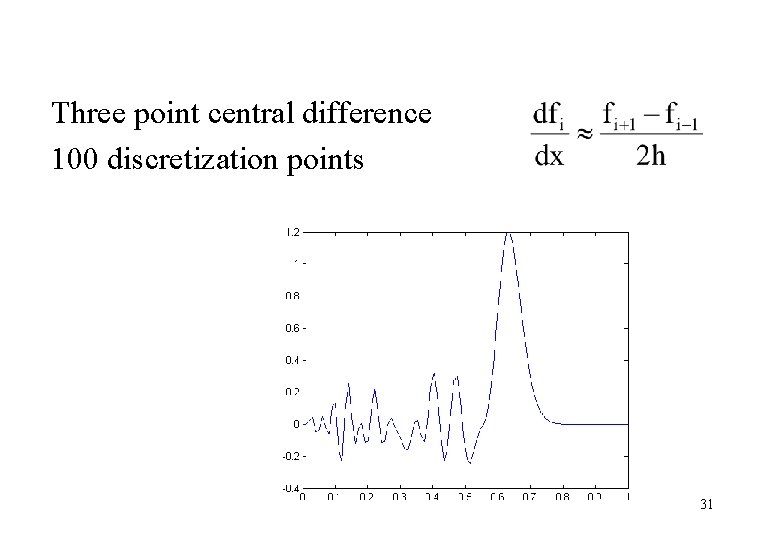
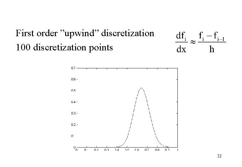
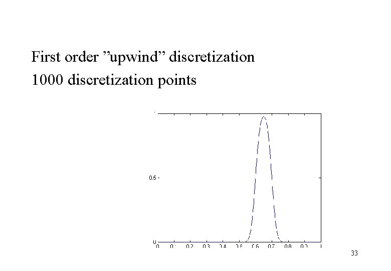
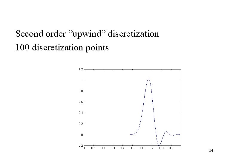
Advection equation example Discretized with interval [0, 1], v=1 m/s, t=0. 5 s Concentration initially everywhere zero but on the interval [0. 1, 0. 2] What does analytical solution predict? 29

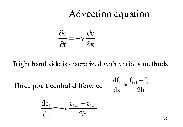
Advection equation Right hand side is discretized with various methods. Three point central difference 30

Three point central difference 100 discretization points 31

First order ”upwind” discretization 100 discretization points 32

First order ”upwind” discretization 1000 discretization points 33

Second order ”upwind” discretization 100 discretization points 34

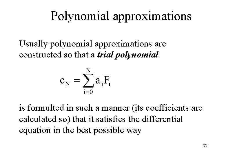
Polynomial approximations Usually polynomial approximations are constructed so that a trial polynomial is formulted in such a manner (its coefficients are calculated so) that it satisfies the differential equation in the best possible way 35

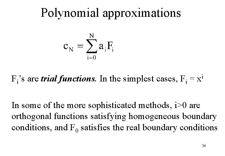
Polynomial approximations Fi’s are trial functions. In the simplest cases, Fi = xi In some of the more sophisticated methods, i>0 are orthogonal functions satisfying homogeneous boundary conditions, and F 0 satisfies the real boundary conditions 36

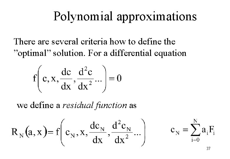
Polynomial approximations There are several criteria how to define the ”optimal” solution. For a differential equation we define a residual function as 37

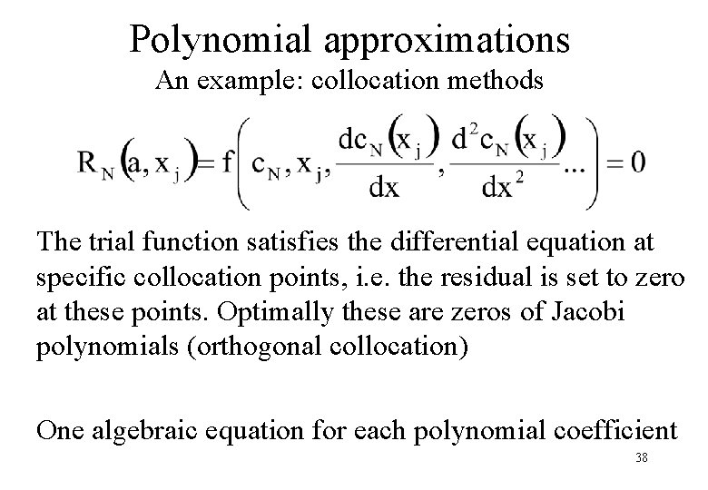
Polynomial approximations An example: collocation methods The trial function satisfies the differential equation at specific collocation points, i. e. the residual is set to zero at these points. Optimally these are zeros of Jacobi polynomials (orthogonal collocation) One algebraic equation for each polynomial coefficient 38

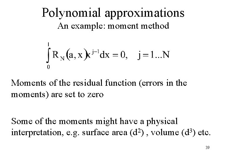
Polynomial approximations An example: moment method Moments of the residual function (errors in the moments) are set to zero Some of the moments might have a physical interpretation, e. g. surface area (d 2) , volume (d 3) etc. 39

40

Some other polynomial approximations • Subdomain method • Galerkin method ( FEM) • Least squares method 41

Finite volume methods (FVM) The basic idea is to formulate balances for a finite volume instead of a differential volume element Also called as ”integral form” of balances Often used in Computational Fluid Dynamics (CFD) 42

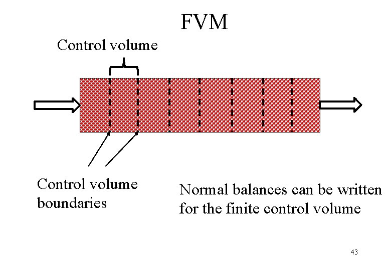
FVM Control volume boundaries Normal balances can be written for the finite control volume 43

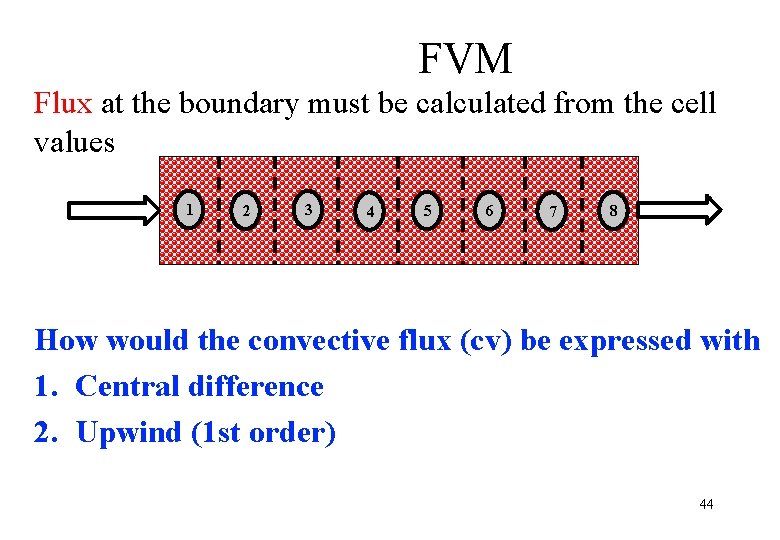
FVM Flux at the boundary must be calculated from the cell values 1 2 3 4 5 6 7 8 How would the convective flux (cv) be expressed with 1. Central difference 2. Upwind (1 st order) 44

Summary • Real modeling problems often lead to partial differential equations, but by assuming symmetries models can be simplified • In coupled problems, variables affect each other. For example reaction rate and temperature • There are many solution methods for partial differential equations. These bring them to a set of ordinary differential equations or algebraic equations • Some solution methods: – Finite difference method – Polynomial approximations – Finite volume method 45