Improve Phase Process Modeling Regression Process Modeling Welcome

Improve Phase Process Modeling Regression

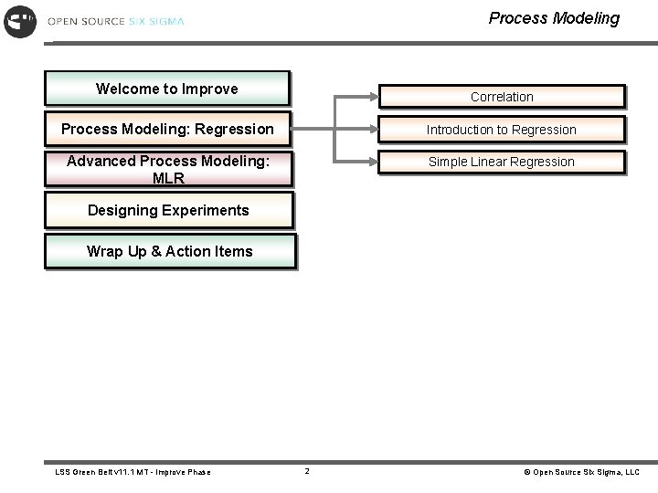
Process Modeling Welcome to Improve Correlation Process Modeling: Regression Introduction to Regression Advanced Process Modeling: MLR Simple Linear Regression Designing Experiments Wrap Up & Action Items LSS Green Belt v 11. 1 MT - Improve Phase 2 © Open Source Six Sigma, LLC

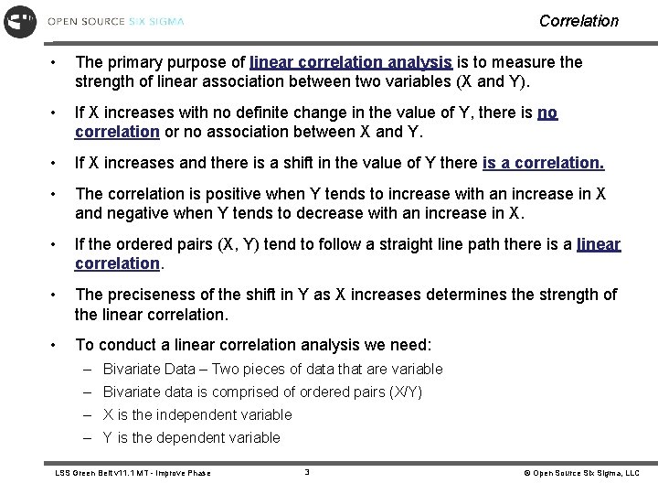
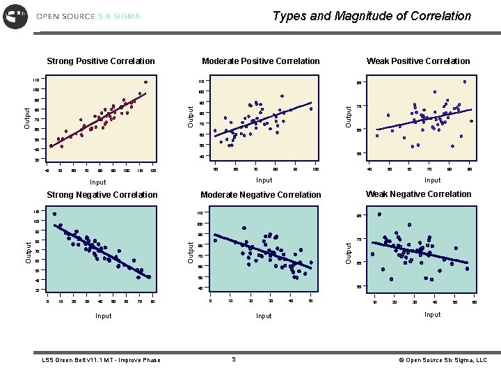
Correlation • The primary purpose of linear correlation analysis is to measure the strength of linear association between two variables (X and Y). • If X increases with no definite change in the value of Y, there is no correlation or no association between X and Y. • If X increases and there is a shift in the value of Y there is a correlation. • The correlation is positive when Y tends to increase with an increase in X and negative when Y tends to decrease with an increase in X. • If the ordered pairs (X, Y) tend to follow a straight line path there is a linear correlation. • The preciseness of the shift in Y as X increases determines the strength of the linear correlation. • To conduct a linear correlation analysis we need: – Bivariate Data – Two pieces of data that are variable – Bivariate data is comprised of ordered pairs (X/Y) – X is the independent variable – Y is the dependent variable LSS Green Belt v 11. 1 MT - Improve Phase 3 © Open Source Six Sigma, LLC

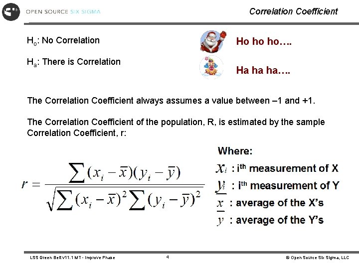
Correlation Coefficient Ho: No Correlation Ho ho ho…. Ha: There is Correlation Ha ha ha…. The Correlation Coefficient always assumes a value between – 1 and +1. The Correlation Coefficient of the population, R, is estimated by the sample Correlation Coefficient, r: LSS Green Belt v 11. 1 MT - Improve Phase 4 © Open Source Six Sigma, LLC

Types and Magnitude of Correlation Moderate Positive Correlation Strong Positive Correlation 110 100 85 100 90 80 70 60 Output 90 Output Weak Positive Correlation 80 70 75 65 60 50 50 40 55 40 30 40 50 60 70 80 90 100 110 50 120 60 70 90 40 100 50 60 70 Input Strong Negative Correlation 90 Weak Negative Correlation 110 100 80 Input Moderate Negative Correlation 110 85 100 90 90 70 60 75 80 Output 80 70 60 50 65 50 40 55 40 30 0 10 20 30 40 50 60 70 80 0 10 Input LSS Green Belt v 11. 1 MT - Improve Phase 20 30 Input 5 40 50 10 20 30 40 50 60 Input © Open Source Six Sigma, LLC

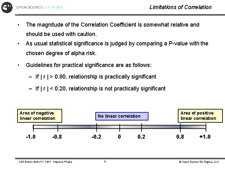
Limitations of Correlation • The magnitude of the Correlation Coefficient is somewhat relative and should be used with caution. • As usual statistical significance is judged by comparing a P-value with the chosen degree of alpha risk. • Guidelines for practical significance are as follows: – If | r | > 0. 80, relationship is practically significant – If | r | < 0. 20, relationship is not practically significant Area of negative linear correlation -1. 0 -0. 8 LSS Green Belt v 11. 1 MT - Improve Phase No linear correlation -0. 2 0 6 0. 2 Area of positive linear correlation 0. 8 +1. 0 © Open Source Six Sigma, LLC

Correlation Example RB Stats Correlation. mtw The Correlation Coefficient [r]: • Is a positive value if one variable increases as the other variable increases. • Is a negative value if one variable decreases as the other increases. Correlation Formula LSS Green Belt v 11. 1 MT - Improve Phase 7 X values Y values Payton carries Payton yards 196 679 311 1390 339 1852 333 1359 369 1610 317 1460 339 1222 148 596 314 1421 381 1684 324 1551 321 1333 146 586 © Open Source Six Sigma, LLC

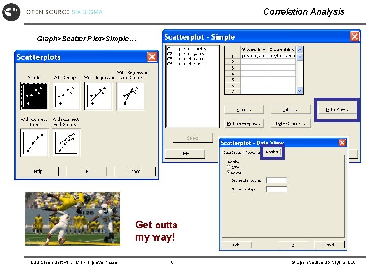
Correlation Analysis Graph>Scatter Plot>Simple… Get outta my way! LSS Green Belt v 11. 1 MT - Improve Phase 8 © Open Source Six Sigma, LLC

Correlation Example Look at the graph. Do you observe any correlation in this graph? Lowess stands for LOcally-WEighted Scatterplot Smoother. LSS Green Belt v 11. 1 MT - Improve Phase 9 © Open Source Six Sigma, LLC

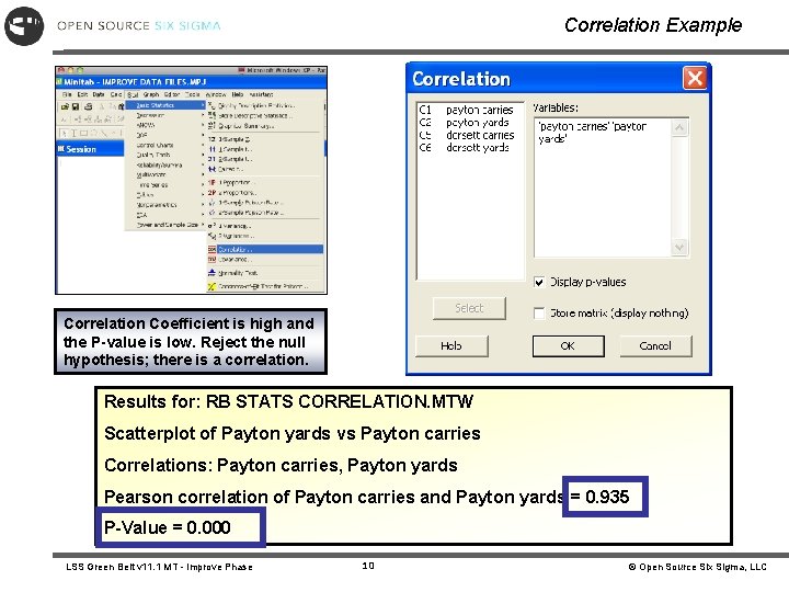
Correlation Example Correlation Coefficient is high and the P-value is low. Reject the null hypothesis; there is a correlation. Results for: RB STATS CORRELATION. MTW Scatterplot of Payton yards vs Payton carries Correlations: Payton carries, Payton yards Pearson correlation of Payton carries and Payton yards = 0. 935 P-Value = 0. 000 LSS Green Belt v 11. 1 MT - Improve Phase 10 © Open Source Six Sigma, LLC

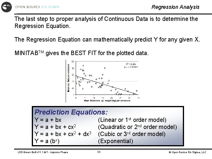
Regression Analysis The last step to proper analysis of Continuous Data is to determine the Regression Equation. The Regression Equation can mathematically predict Y for any given X. MINITABTM gives the BEST FIT for the plotted data. Prediction Equations: Y = a + bx + cx 2 + dx 3 Y = a (bx) LSS Green Belt v 11. 1 MT - Improve Phase (Linear or 1 st order model) (Quadratic or 2 nd order model) (Cubic or 3 rd order model) (Exponential) 11 © Open Source Six Sigma, LLC

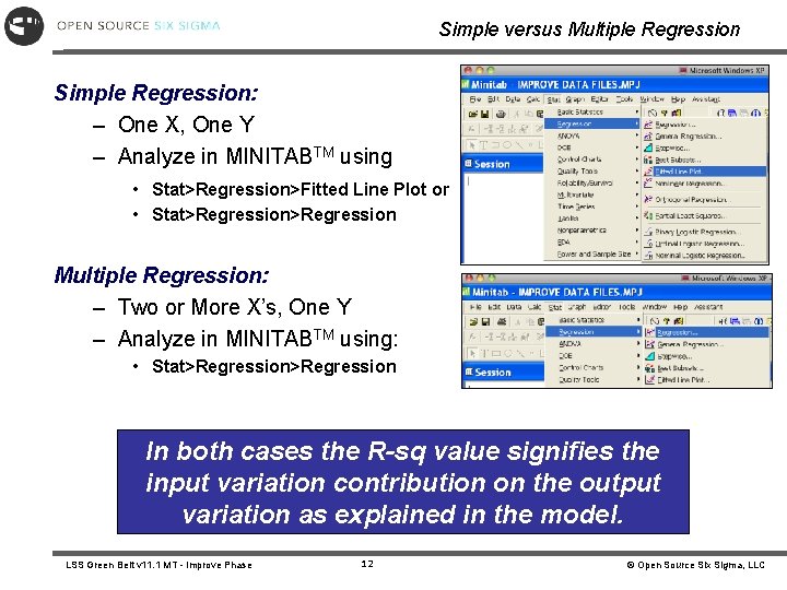
Simple versus Multiple Regression Simple Regression: – One X, One Y – Analyze in MINITABTM using • Stat>Regression>Fitted Line Plot or • Stat>Regression Multiple Regression: – Two or More X’s, One Y – Analyze in MINITABTM using: • Stat>Regression In both cases the R-sq value signifies the input variation contribution on the output variation as explained in the model. LSS Green Belt v 11. 1 MT - Improve Phase 12 © Open Source Six Sigma, LLC

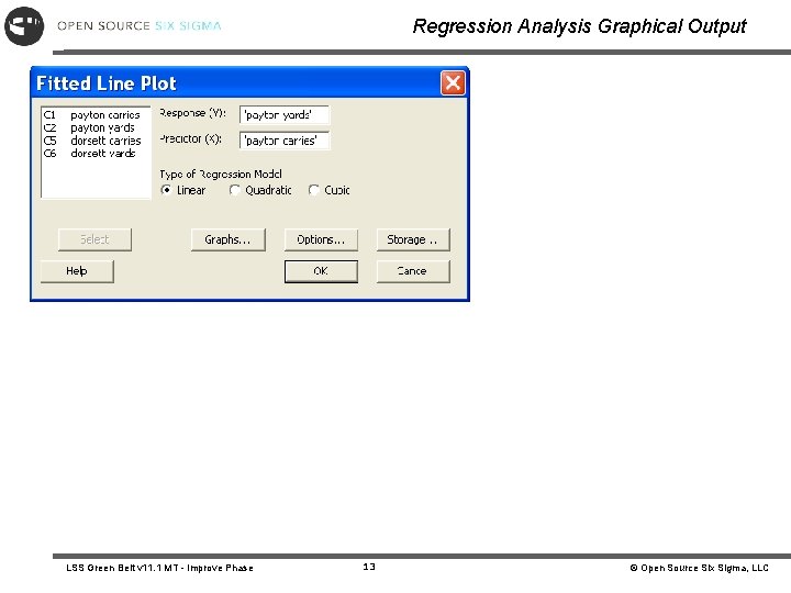
Regression Analysis Graphical Output LSS Green Belt v 11. 1 MT - Improve Phase 13 © Open Source Six Sigma, LLC

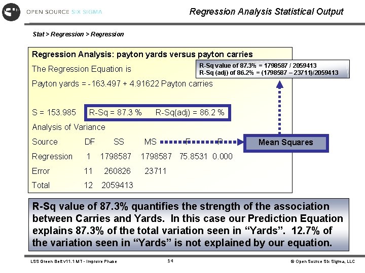
Regression Analysis Statistical Output Stat > Regression Analysis: payton yards versus payton carries R-Sq value of 87. 3% = 1798587 / 2059413 R-Sq (adj) of 86. 2% = (1798587 – 23711)/2059413 The Regression Equation is Payton yards = -163. 497 + 4. 91622 Payton carries S = 153. 985 R-Sq = 87. 3 % R-Sq(adj) = 86. 2 % Analysis of Variance Source DF SS Regression 1 1798587 Error 11 260826 Total 12 2059413 MS F P Mean Squares 1798587 75. 8531 0. 000 23711 R-Sq value of 87. 3% quantifies the strength of the association between Carries and Yards. In this case our Prediction Equation explains 87. 3% of the total variation seen in “Yards”. 12. 7% of the variation seen in “Yards” is not explained by our equation. LSS Green Belt v 11. 1 MT - Improve Phase 14 © Open Source Six Sigma, LLC

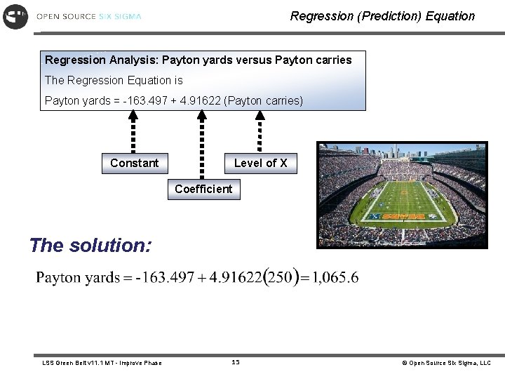
Regression (Prediction) Equation Regression Analysis: Payton yards versus Payton carries The Regression Equation is Payton yards = -163. 497 + 4. 91622 (Payton carries) Constant Level of X Coefficient The solution: LSS Green Belt v 11. 1 MT - Improve Phase 15 © Open Source Six Sigma, LLC

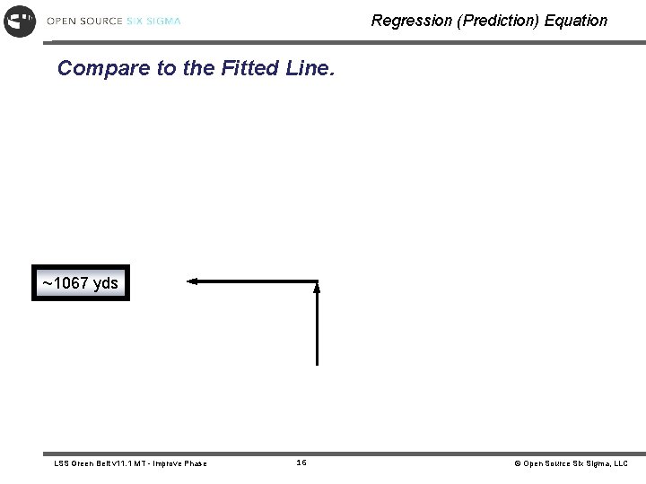
Regression (Prediction) Equation Compare to the Fitted Line. ~1067 yds LSS Green Belt v 11. 1 MT - Improve Phase 16 © Open Source Six Sigma, LLC

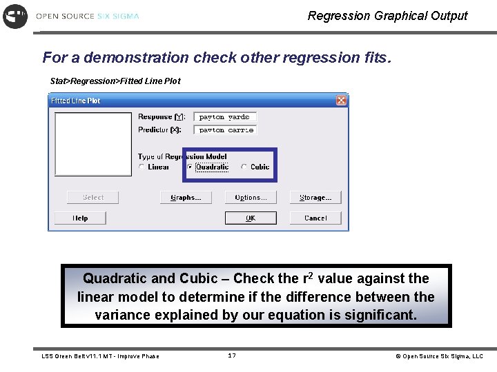
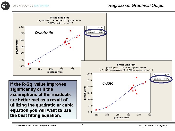
Regression Graphical Output For a demonstration check other regression fits. Stat>Regression>Fitted Line Plot Quadratic and Cubic – Check the r 2 value against the linear model to determine if the difference between the variance explained by our equation is significant. LSS Green Belt v 11. 1 MT - Improve Phase 17 © Open Source Six Sigma, LLC

Regression Graphical Output Quadratic Cubic If the R-Sq value improves significantly or if the assumptions of the residuals are better met as a result of utilizing the quadratic or cubic equation you will want to use the best fitting equation. LSS Green Belt v 11. 1 MT - Improve Phase 18 © Open Source Six Sigma, LLC

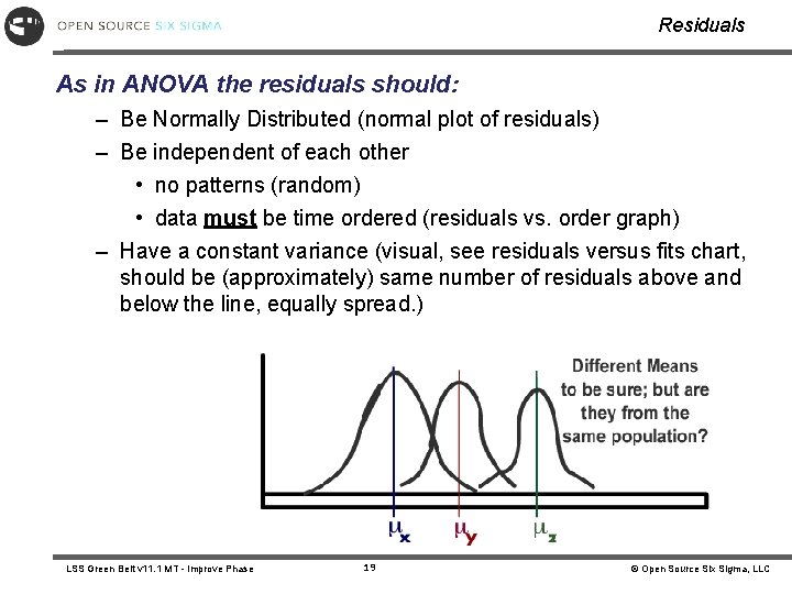
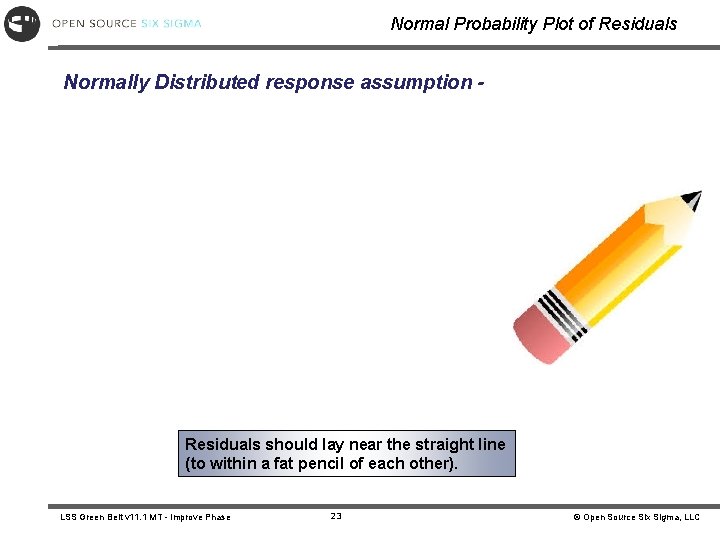
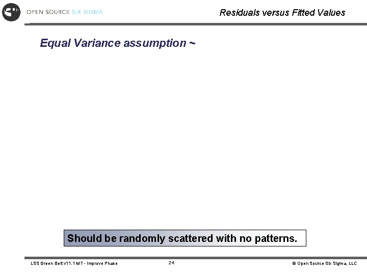
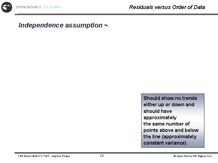
Residuals As in ANOVA the residuals should: – Be Normally Distributed (normal plot of residuals) – Be independent of each other • no patterns (random) • data must be time ordered (residuals vs. order graph) – Have a constant variance (visual, see residuals versus fits chart, should be (approximately) same number of residuals above and below the line, equally spread. ) LSS Green Belt v 11. 1 MT - Improve Phase 19 © Open Source Six Sigma, LLC

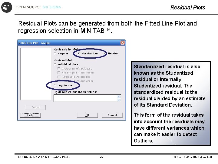
Residual Plots can be generated from both the Fitted Line Plot and regression selection in MINITABTM. Standardized residual is also known as the Studentized residual or internally Studentized residual. The standardized residual is the residual divided by an estimate of its Standard Deviation. This form of the residual takes into account the residuals may have different variances which can make it easier to detect Outliers. LSS Green Belt v 11. 1 MT - Improve Phase 20 © Open Source Six Sigma, LLC

Residuals Equal variance assumption… Normality assumption… Independence assumption… LSS Green Belt v 11. 1 MT - Improve Phase 21 © Open Source Six Sigma, LLC

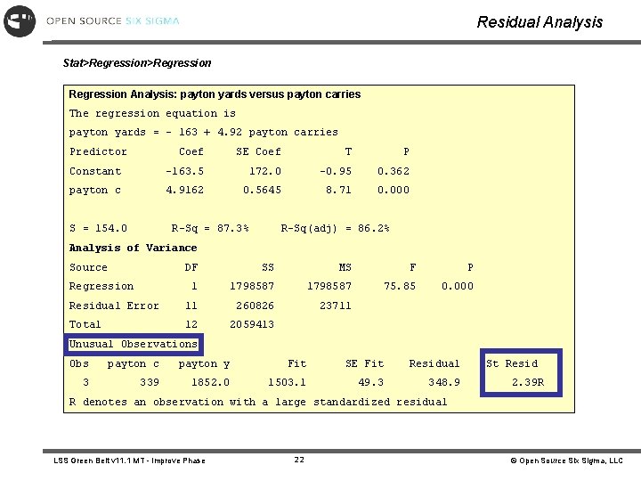
Residual Analysis Stat>Regression Analysis: payton yards versus payton carries The regression equation is payton yards = - 163 + 4. 92 payton carries Predictor Coef SE Coef T P Constant -163. 5 172. 0 -0. 95 0. 362 payton c 4. 9162 0. 5645 8. 71 0. 000 S = 154. 0 R-Sq = 87. 3% R-Sq(adj) = 86. 2% Analysis of Variance Source DF SS MS F P 1 1798587 75. 85 0. 000 Residual Error 11 260826 23711 Total 12 2059413 Regression Unusual Observations Obs payton c payton y Fit SE Fit Residual 3 339 1852. 0 1503. 1 49. 3 348. 9 St Resid 2. 39 R R denotes an observation with a large standardized residual LSS Green Belt v 11. 1 MT - Improve Phase 22 © Open Source Six Sigma, LLC

Normal Probability Plot of Residuals Normally Distributed response assumption - Residuals should lay near the straight line (to within a fat pencil of each other). LSS Green Belt v 11. 1 MT - Improve Phase 23 © Open Source Six Sigma, LLC

Residuals versus Fitted Values Equal Variance assumption ~ Should be randomly scattered with no patterns. LSS Green Belt v 11. 1 MT - Improve Phase 24 © Open Source Six Sigma, LLC

Residuals versus Order of Data Independence assumption ~ Should show no trends either up or down and should have approximately the same number of points above and below the line (approximately constant variance). LSS Green Belt v 11. 1 MT - Improve Phase 25 © Open Source Six Sigma, LLC

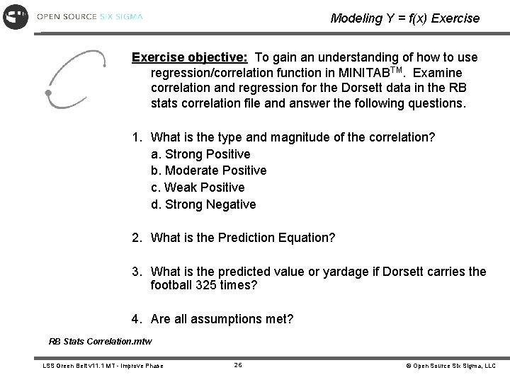
Modeling Y = f(x) Exercise objective: To gain an understanding of how to use regression/correlation function in MINITABTM. Examine correlation and regression for the Dorsett data in the RB stats correlation file and answer the following questions. 1. What is the type and magnitude of the correlation? a. Strong Positive b. Moderate Positive c. Weak Positive d. Strong Negative 2. What is the Prediction Equation? 3. What is the predicted value or yardage if Dorsett carries the football 325 times? 4. Are all assumptions met? RB Stats Correlation. mtw LSS Green Belt v 11. 1 MT - Improve Phase 26 © Open Source Six Sigma, LLC

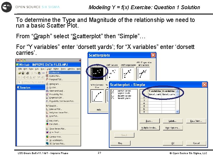
Modeling Y = f(x) Exercise: Question 1 Solution To determine the Type and Magnitude of the relationship we need to run a basic Scatter Plot. From “Graph” select “Scatterplot” then “Simple”… For “Y variables” enter ‘dorsett yards’; for “X variables” enter ‘dorsett carries’. LSS Green Belt v 11. 1 MT - Improve Phase 27 © Open Source Six Sigma, LLC

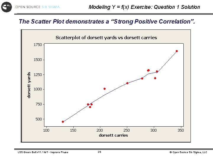
Modeling Y = f(x) Exercise: Question 1 Solution The Scatter Plot demonstrates a “Strong Positive Correlation”. LSS Green Belt v 11. 1 MT - Improve Phase 28 © Open Source Six Sigma, LLC

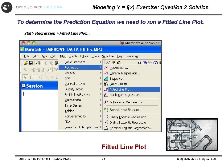
Modeling Y = f(x) Exercise: Question 2 Solution To determine the Prediction Equation we need to run a Fitted Line Plot. Stat > Regression > Fitted Line Plot… Fitted Line Plot LSS Green Belt v 11. 1 MT - Improve Phase 29 © Open Source Six Sigma, LLC

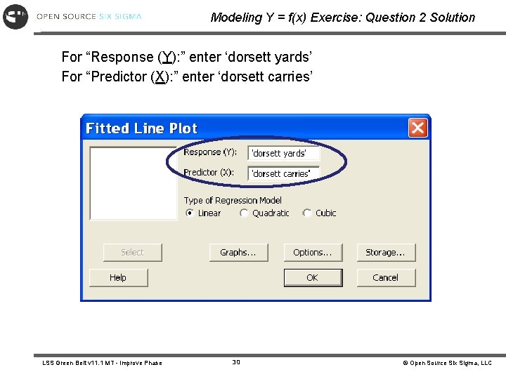
Modeling Y = f(x) Exercise: Question 2 Solution For “Response (Y): ” enter ‘dorsett yards’ For “Predictor (X): ” enter ‘dorsett carries’ LSS Green Belt v 11. 1 MT - Improve Phase 30 © Open Source Six Sigma, LLC

Modeling Y = f(x) Exercise: Question 2 Solution The Prediction Equation is shown here… LSS Green Belt v 11. 1 MT - Improve Phase 31 © Open Source Six Sigma, LLC

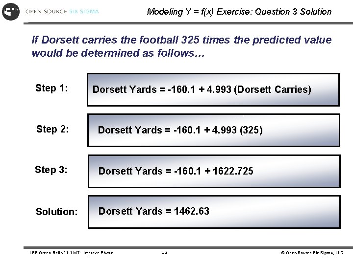
Modeling Y = f(x) Exercise: Question 3 Solution If Dorsett carries the football 325 times the predicted value would be determined as follows… Step 1: Dorsett Yards = -160. 1 + 4. 993 (Dorsett Carries) Step 2: Dorsett Yards = -160. 1 + 4. 993 (325) Step 3: Dorsett Yards = -160. 1 + 1622. 725 Solution: Dorsett Yards = 1462. 63 LSS Green Belt v 11. 1 MT - Improve Phase 32 © Open Source Six Sigma, LLC

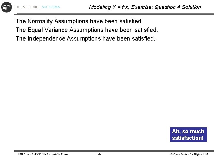
Modeling Y = f(x) Exercise: Question 4 Solution The Normality Assumptions have been satisfied. The Equal Variance Assumptions have been satisfied. The Independence Assumptions have been satisfied. Ah, so much satisfaction! LSS Green Belt v 11. 1 MT - Improve Phase 33 © Open Source Six Sigma, LLC

Summary At this point you should be able to: § Perform the steps in a Correlation and a Regression Analysis § Explain when Correlation and Regression is appropriate LSS Green Belt v 11. 1 MT - Improve Phase 34 © Open Source Six Sigma, LLC

LSS Green Belt v 11. 1 MT - Improve Phase © Open Source Six Sigma, LLC