Chapter 3 QUADRATIC FUNCTIONS Section 3 1 Introduction

Chapter 3 QUADRATIC FUNCTIONS Section 3. 1 Introduction to the Family of Quadratic Functions Section 3. 2 The Vertex of a Parabola Functions Modeling Change: A Preparation for Calculus, 5 th Edition, 2014, Connally 1

3. 1 INTRODUCTION TO THE FAMILY OF QUADRATIC FUNCTIONS Functions Modeling Change: A Preparation for Calculus, 5 th Edition, 2014, Connally 2

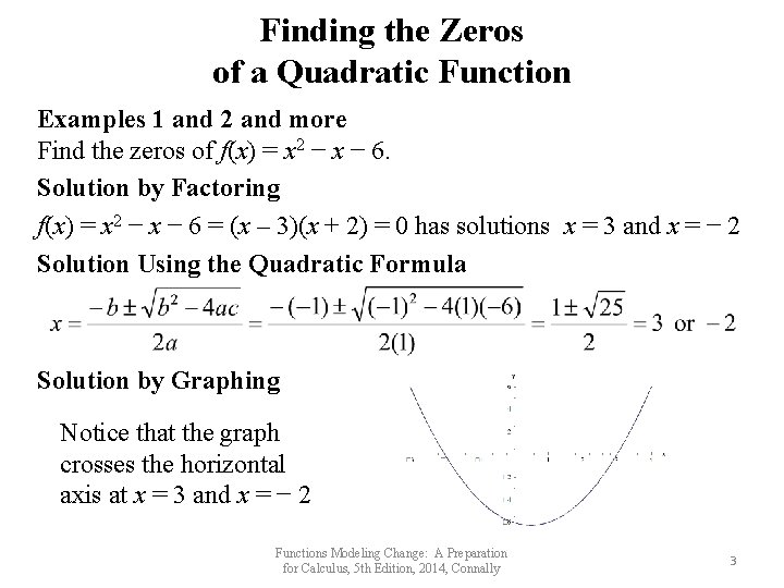
Finding the Zeros of a Quadratic Function Examples 1 and 2 and more Find the zeros of f(x) = x 2 − x − 6. Solution by Factoring f(x) = x 2 − x − 6 = (x – 3)(x + 2) = 0 has solutions x = 3 and x = − 2 Solution Using the Quadratic Formula Solution by Graphing Notice that the graph crosses the horizontal axis at x = 3 and x = − 2 Functions Modeling Change: A Preparation for Calculus, 5 th Edition, 2014, Connally 3

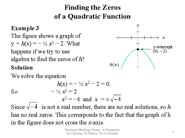
Finding the Zeros of a Quadratic Function Example 3 The figure shows a graph of y = h(x) = − ½ x 2 − 2. What happens if we try to use algebra to find the zeros of h? Solution We solve the equation h(x) = − ½ x 2 − 2 = 0. So − ½ x 2 = 2 x 2 = − 4 and x = ± Since is not a real number, there are no real solutions, so h has no real zeros. This corresponds to the fact that the graph of h in the figure does not cross the x-axis. Functions Modeling Change: A Preparation for Calculus, 5 th Edition, 2014, Connally 4

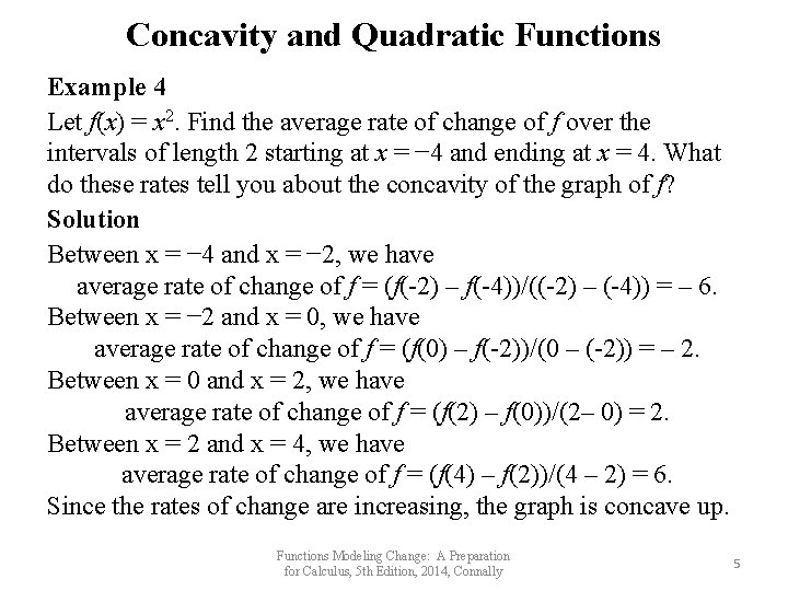
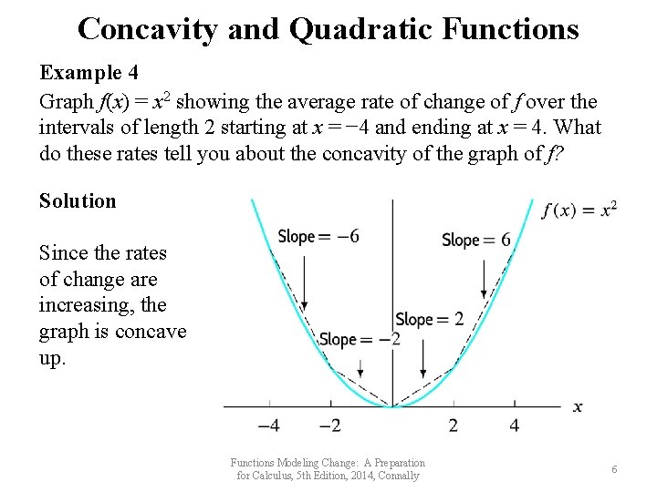
Concavity and Quadratic Functions Example 4 Let f(x) = x 2. Find the average rate of change of f over the intervals of length 2 starting at x = − 4 and ending at x = 4. What do these rates tell you about the concavity of the graph of f? Solution Between x = − 4 and x = − 2, we have average rate of change of f = (f(-2) – f(-4))/((-2) – (-4)) = – 6. Between x = − 2 and x = 0, we have average rate of change of f = (f(0) – f(-2))/(0 – (-2)) = – 2. Between x = 0 and x = 2, we have average rate of change of f = (f(2) – f(0))/(2– 0) = 2. Between x = 2 and x = 4, we have average rate of change of f = (f(4) – f(2))/(4 – 2) = 6. Since the rates of change are increasing, the graph is concave up. Functions Modeling Change: A Preparation for Calculus, 5 th Edition, 2014, Connally 5

Concavity and Quadratic Functions Example 4 Graph f(x) = x 2 showing the average rate of change of f over the intervals of length 2 starting at x = − 4 and ending at x = 4. What do these rates tell you about the concavity of the graph of f? Solution Since the rates of change are increasing, the graph is concave up. Functions Modeling Change: A Preparation for Calculus, 5 th Edition, 2014, Connally 6

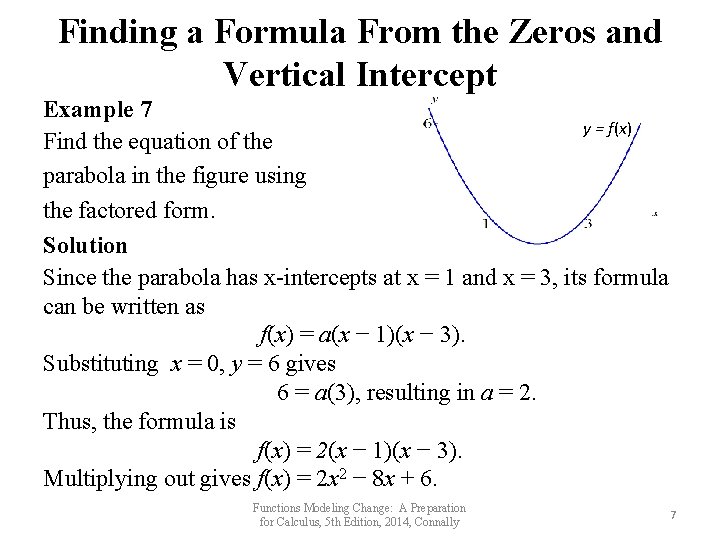
Finding a Formula From the Zeros and Vertical Intercept Example 7 y = f(x) Find the equation of the parabola in the figure using the factored form. Solution Since the parabola has x-intercepts at x = 1 and x = 3, its formula can be written as f(x) = a(x − 1)(x − 3). Substituting x = 0, y = 6 gives 6 = a(3), resulting in a = 2. Thus, the formula is f(x) = 2(x − 1)(x − 3). Multiplying out gives f(x) = 2 x 2 − 8 x + 6. Functions Modeling Change: A Preparation for Calculus, 5 th Edition, 2014, Connally 7

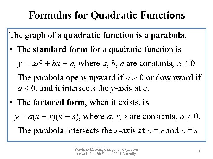
Formulas for Quadratic Functions The graph of a quadratic function is a parabola. • The standard form for a quadratic function is y = ax 2 + bx + c, where a, b, c are constants, a ≠ 0. The parabola opens upward if a > 0 or downward if a < 0, and it intersects the y-axis at c. • The factored form, when it exists, is y = a(x − r)(x − s), where a, r, s are constants, a ≠ 0. The parabola intersects the x-axis at x = r and x = s. Functions Modeling Change: A Preparation for Calculus, 5 th Edition, 2014, Connally 8

3. 2 THE VERTEX OF A PARABOLA Functions Modeling Change: A Preparation for Calculus, 5 th Edition, 2014, Connally 9

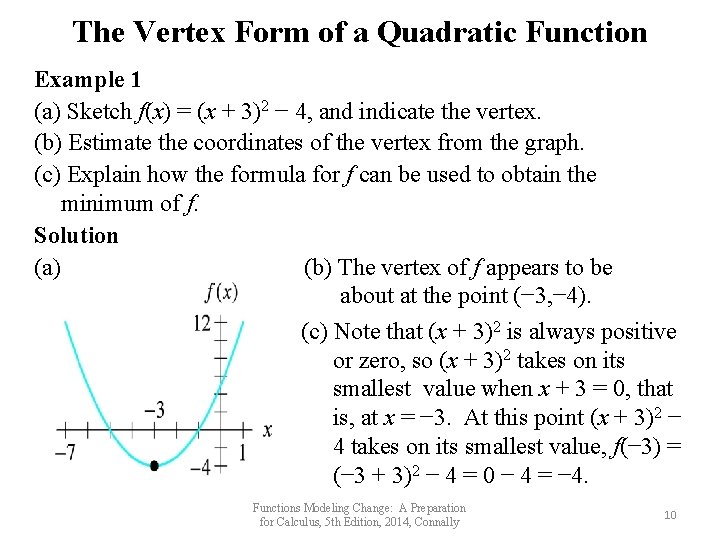
The Vertex Form of a Quadratic Function Example 1 (a) Sketch f(x) = (x + 3)2 − 4, and indicate the vertex. (b) Estimate the coordinates of the vertex from the graph. (c) Explain how the formula for f can be used to obtain the minimum of f. Solution (a) (b) The vertex of f appears to be about at the point (− 3, − 4). (c) Note that (x + 3)2 is always positive or zero, so (x + 3)2 takes on its smallest value when x + 3 = 0, that is, at x = − 3. At this point (x + 3)2 − 4 takes on its smallest value, f(− 3) = (− 3 + 3)2 − 4 = 0 − 4 = − 4. Functions Modeling Change: A Preparation for Calculus, 5 th Edition, 2014, Connally 10

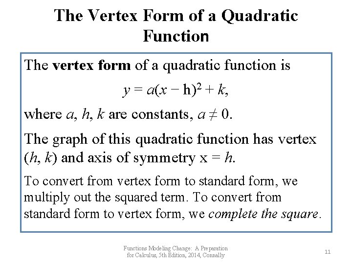
The Vertex Form of a Quadratic Function The vertex form of a quadratic function is y = a(x − h)2 + k, where a, h, k are constants, a ≠ 0. The graph of this quadratic function has vertex (h, k) and axis of symmetry x = h. To convert from vertex form to standard form, we multiply out the squared term. To convert from standard form to vertex form, we complete the square. Functions Modeling Change: A Preparation for Calculus, 5 th Edition, 2014, Connally 11

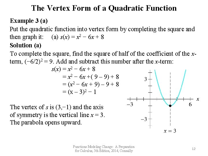
The Vertex Form of a Quadratic Function Example 3 (a) Put the quadratic function into vertex form by completing the square and then graph it: (a) s(x) = x 2 − 6 x + 8 Solution (a) To complete the square, find the square of half of the coefficient of the xterm, (− 6/2)2 = 9. Add and subtract this number after the x-term: s(x) = x 2 − 6 x + 8 = x 2 − 6 x +( 9 – 9) + 8 = (x 2 − 6 x + 9) – 9 + 8 = (x – 3)2 − 1 The vertex of s is (3, − 1) and the axis of symmetry is the vertical line x = 3. The parabola opens upward. Functions Modeling Change: A Preparation for Calculus, 5 th Edition, 2014, Connally 12

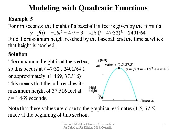
Modeling with Quadratic Functions Example 5 For t in seconds, the height of a baseball in feet is given by the formula y = f(t) = − 16 t 2 + 47 t + 3 = -16 (t – 47/32)2. – 2401/64 Find the maximum height reached by the baseball and the time at whick that height is reached. Solution The maximum height is at the vertex, so this occurs at ( 47/32 , 2401/64 ), or approximately (1. 469, 37. 516). This means that the ball reaches its maximum height of 37. 516 feet at t = 1. 469 seconds. Note that these values are close to the graphical estimates (1. 5, 37. 5) made at the beginning of this section. Functions Modeling Change: A Preparation for Calculus, 5 th Edition, 2014, Connally 13