Chapter 2 Signals and Spectra All sections except

Chapter 2 Signals and Spectra (All sections, except Section 8, are covered. )

Physically Realizable Waveform 1. Non zero over finite duration (finite energy) 2. Non zero over finite frequency range (physical limitation of media) 3. Continuous in time (finite bandwidth) 4. Finite peak value (physical limitation of equipment) 5. Real valued (must be observable)

• Power Signal: finite power, infinite energy • Energy Signal: finite energy, non-zero power over limited time • All physical signals are energy signals. Nothing can have infinite power. However, mathematically it is more convenient to deal with power signals. We will use power signals to approximate the behavior of energy signals over the time intervals of interest.

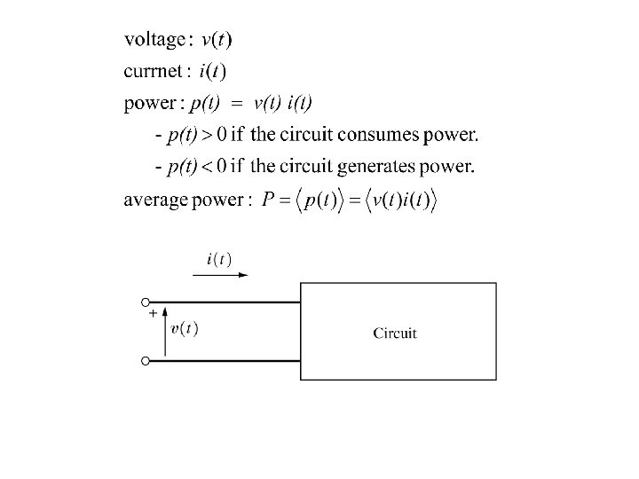
i(t) R + v(t) -

power in System signal, s(t) noise, n(t) power out System

The phasor is a complex number that carries the amplitude and phase angle information of a sinusoidal function. It does not include the angular frequency. Euler’s identify : Given

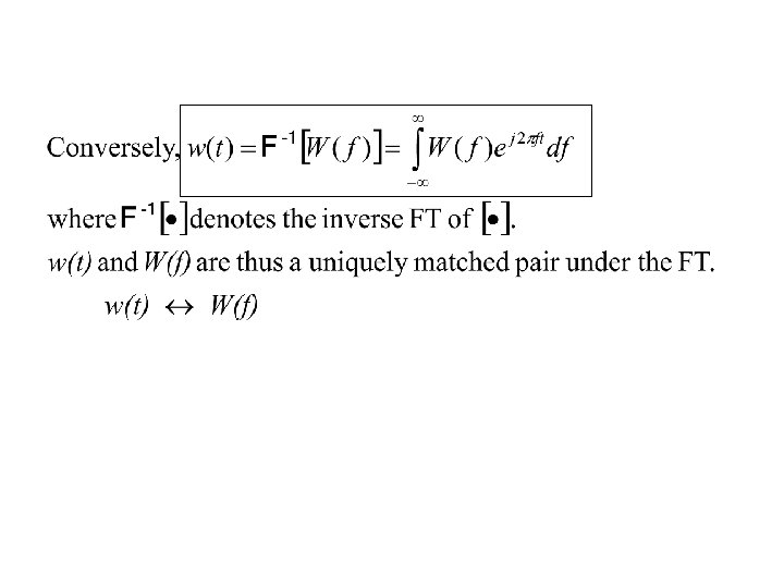
Fourier Transform Signal is a measurable, physical quantity which carries information. In time, it is quantified as w(t). Sometimes it is convenient to view through its frequency components. Fourier Transform (FT) is a mathematical tool to identify the presence of frequency component for any wave form.

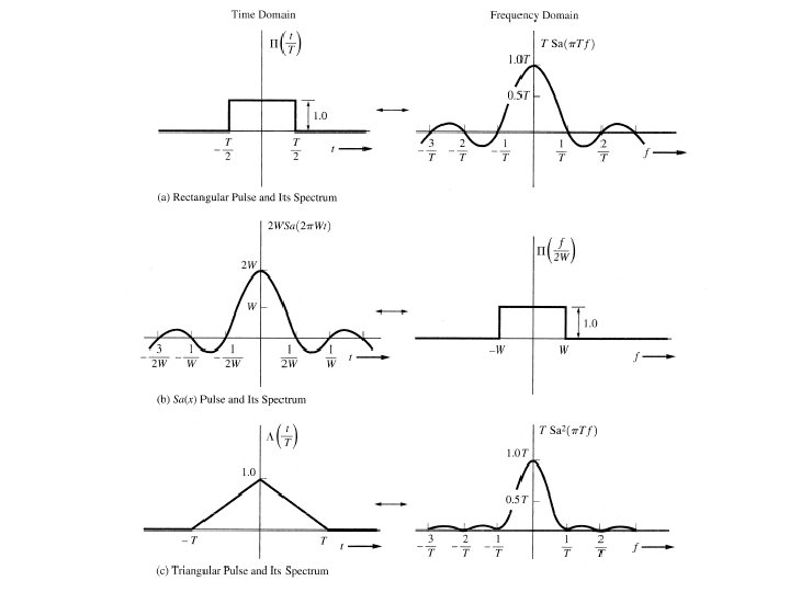
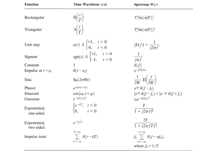
Note: It is in general difficult to evaluate the FT integrations for arbitrary functions. There are certain well known functions used in the FT along with the properties of the FT.

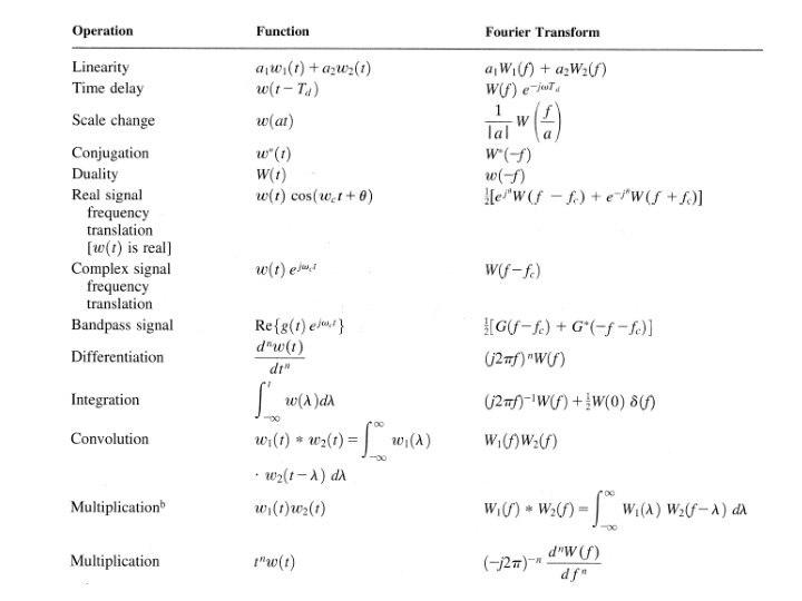
Properties of Fourier Transform If w(t) is real, W(-f) = W*(f). 1. 2. Linearity: a 1 w 1(t)+a 2 w 2(t) a 1 W 1(f) + a 2 W 2(f) 3. Time delay: w(t – T) = W(f) e-j 2 f. T 4. Frequency Translation: w(t) ej 2 fot W(f – fo) 5. Convolution: w 1(t)X w 2(t) W 1(f)W 2(f) 6. Multiplication: w 1(t)w 2(t) W 1(f)X W 2(f) Note: * is complex conjugate. X is convolution integral.

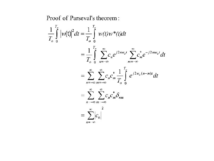
Parseval’s Theorem

Dirac Delta Function

Unit Step Function

More Commonly Used Functions

Spectrum of Sine Wave Couch, Digital and Analog Communication Systems, Seventh Edition © 2007 Pearson Education, Inc. All rights reserved. 0 -13 -142492 -0

Figure 2– 8 Waveform and spectrum of a switched sinusoid. Spectrum of Truncated Sine Wave

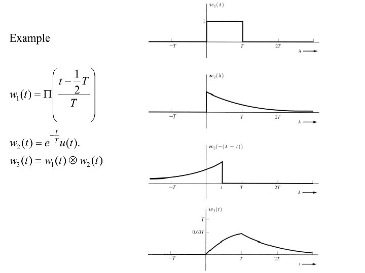
Example: Double Exponential

Convolution Supposed t is fixed at an arbitrary value. Within the integration, w 2(t- ) is a “horizontally flipped about =0, and move to the right by t version” of w 2( ). Now, multiply w 1( ) with w 2(t- ) for each point of . Then, integrate over - < < . The result is w 3(t) for this fixed value of t. Repeat this process for all values of t, - < t < .

Power Spectrum Density

1 w(t) t -1 0 1 w(t+ ) if < -2 t -1 - 0 1 - w(t+ ) if > 2 t -1 - 0 1 - w(t+ ) if -2 < 0 t -1 - 0 1 - w(t+ ) if 0 2 t -1 - 0 1 -

1 -2 2 2 f -1. 5 -1. 0 -0. 5 0 0. 5 1. 0 1. 5

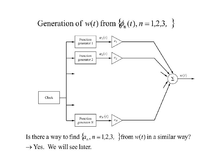
Orthogonal Series Representation

Examples of Orthogonal Functions Sinusoids Polynomials Square Waves

Fourier Series (pages 71 – 78 not covered)

Properties of Fourier Series

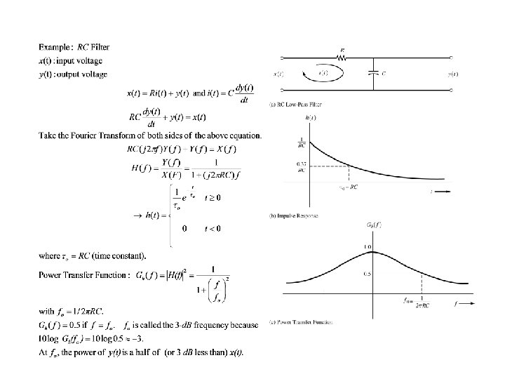
Impulse Response

Distortion

Note: Sections 2. 7 and 2. 9 will be covered briefly. Section 2. 8 will not be covered.

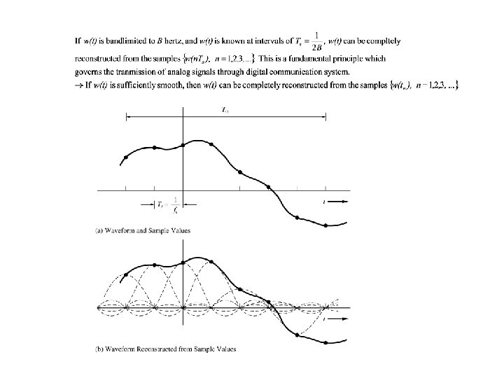
Sampling w(t) t 1 t 2 t 3 t 4 t 5 t

w(t) t 1 t 2 t 3 t 4 t 5 t ws(t) t 1 t 2 t 3 t 4 t 5 t

w(t) sampler (t-n. Ts) ws(t) Low Pass Filter Ideal cutoff at B w(t)

If fs < 2 B, the sampling rate is insufficient, i. e. , there aren’t enough samples to reconstruct the original waveform. Aliasing or spectral folding. The original waveform cannot be reconstructed without distortion.

Dimensionality Theorem For a bandlimited waveform with bandwidth B hertz, if the waveform can be completely specified (i. e. , later reconstructed by an ideal low pass filter) by N=2 BTo samples during a time period of To, then N is the dimension of the wave form. Conversely, to estimate the bandwidth of a waveform, find a number N such that N=2 BTo is the minimum number of samples needed to reconstruct the waveform during a time period To. Then B follows. As To , any approximation goes to zero. A slightly modified version of this theorem is the Bandpass Dimensionality Theorem: Any bandpass waveform (with bandwidth B) can be determined by N=2 BTo samples taken during a period of To.

Data Rate Theorem (Corollary to Dimensionality Theorem) The maximum number of independent quantities which can be transmitted by a bandlimited channel (B hertz) during a time period of To is N=2 BTo. Definition. The baud rate of a digital communication system is the rate of symbols or quantities transmitted per second. From the Data Rate Theorem, the maximum baud rate of a system with a bandlimited channel (B hertz) is 2 B symbols / second. Definition. The data rate (or bit rate), R, of a system is the baud rate times the information content per symbol (H): R= 2 BH bits / second Suppose a source transmits one of M equally likely symbols. The information content of each symbol: H = log 2 (1/probablity of each symbol) = log 2 M R= 2 Blog 2 M Data rate is (also known as the Channel Capacity) is determined by (1) channel bandwidth and (2) channel SNR.