DOPPLER SPECTRA OF WEATHER SIGNALS Chapter 5 examples

DOPPLER SPECTRA OF WEATHER SIGNALS (Chapter 5; examples from chapter 9)

Spectrum and Autocorrelation Skip?

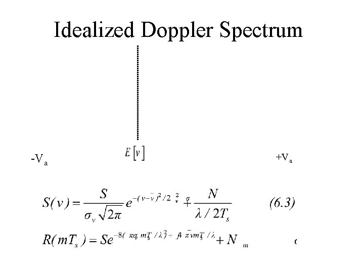
Idealized Doppler Spectrum -Va +Va

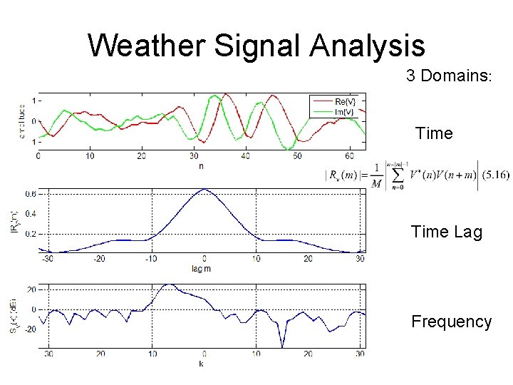
Weather Signal Analysis 3 Domains: Time Lag Frequency

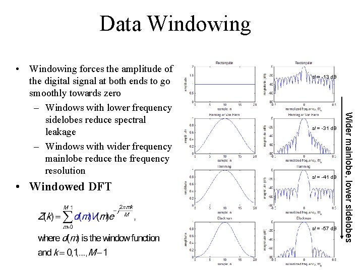
Data Windowing • Windowed DFT sl = -13 d. B sl = -31 d. B sl = -41 d. B sl = -57 d. B Wider mainlobe, lower sidelobes • Windowing forces the amplitude of the digital signal at both ends to go smoothly towards zero – Windows with lower frequency sidelobes reduce spectral leakage – Windows with wider frequency mainlobe reduce the frequency resolution

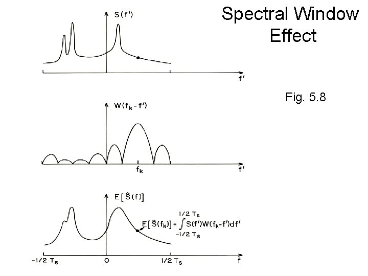
Spectral Window Effect Fig. 5. 8

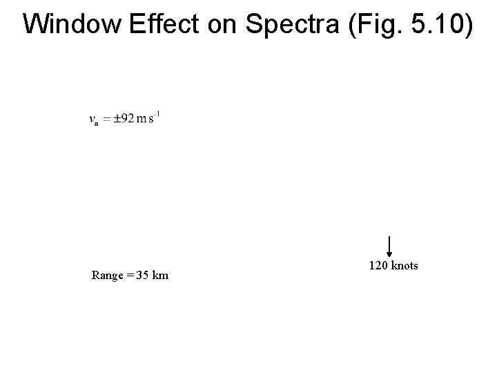
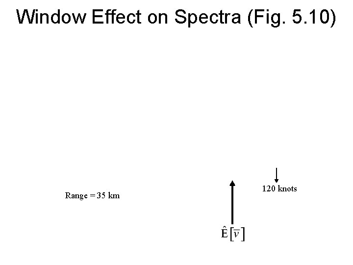
Window Effect on Spectra (Fig. 5. 10) Range = 35 km 120 knots

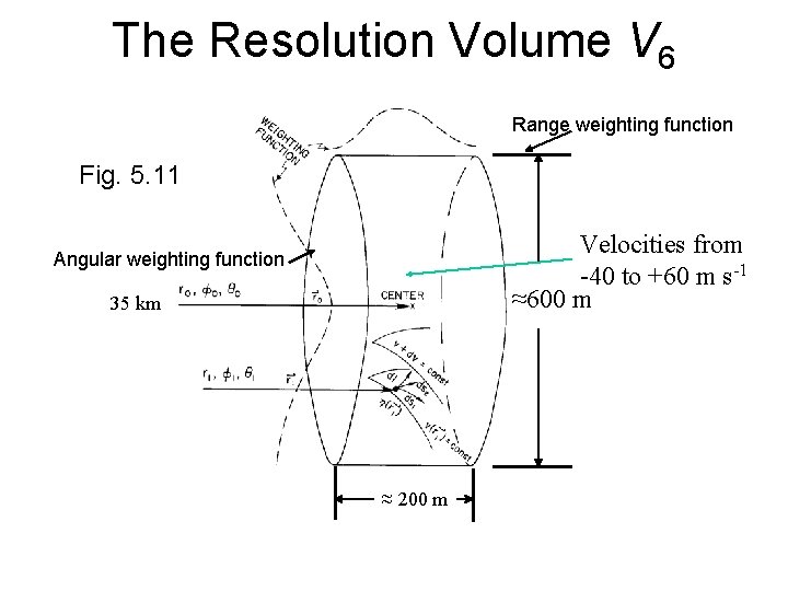
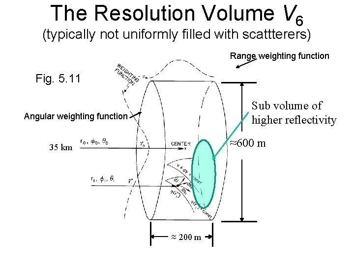
The Resolution Volume V 6 Range weighting function Fig. 5. 11 Velocities from -40 to +60 m s-1 ≈600 m Angular weighting function 35 km ≈ 200 m

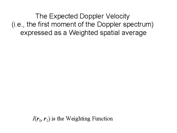
The Expected Doppler Velocity (i. e. , the first moment of the Doppler spectrum) expressed as a Weighted spatial average I(r 0, r 1) is the Weighting Function

The Resolution Volume V 6 (typically not uniformly filled with scattterers) Range weighting function Fig. 5. 11 Sub volume of higher reflectivity Angular weighting function ≈600 m 35 km ≈ 200 m

Window Effect on Spectra (Fig. 5. 10) Range = 35 km 120 knots

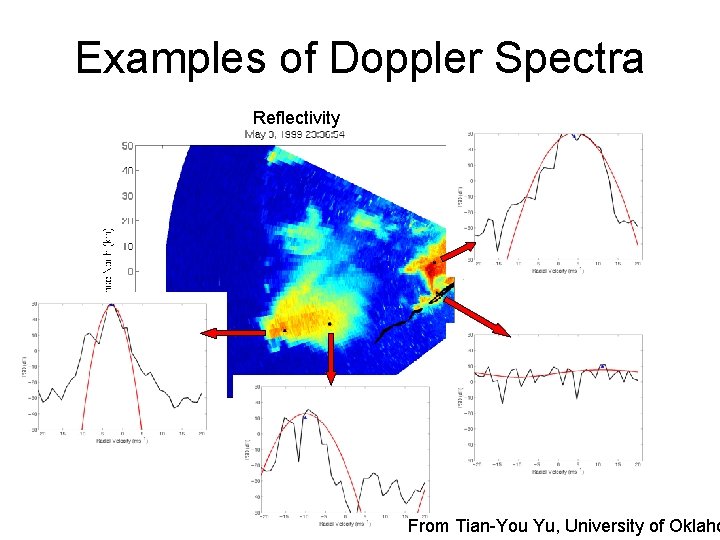
Examples of Doppler Spectra Reflectivity From Tian-You Yu, University of Oklaho

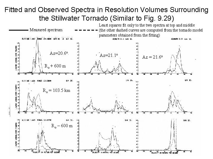
Fitted and Observed Spectra in Resolution Volumes Surrounding the Stillwater Tornado (Similar to Fig. 9. 29) Measured spectrum Az=20. 6 o Ro + 600 m Ro = 103. 5 km Ro – 600 m Least squares fit only to the two spectra at top and middle (the other dashed curves are computed from the tornado model parameters obtained from the fitting) Az=21. 1 o Az = 21. 6 o

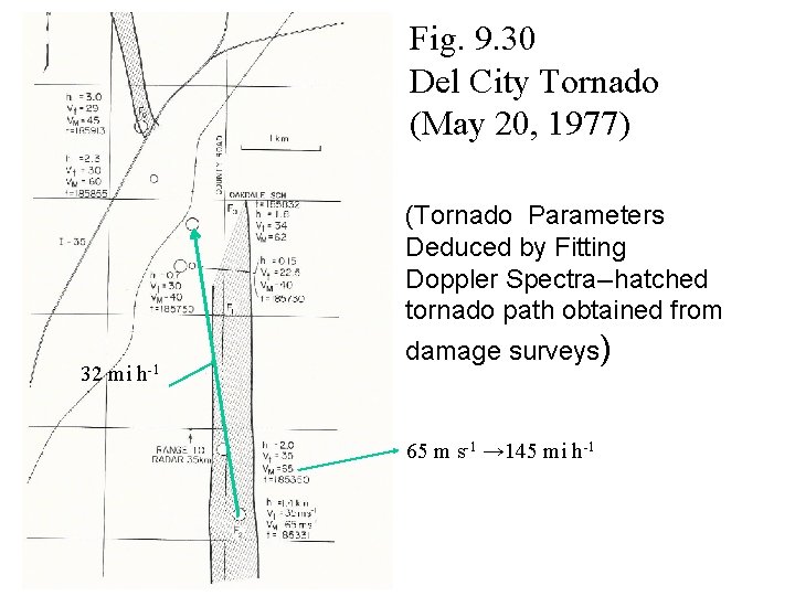
Fig. 9. 30 Del City Tornado (May 20, 1977) (Tornado Parameters Deduced by Fitting Doppler Spectra--hatched tornado path obtained from 32 mi h-1 damage surveys) 65 m s-1 → 145 mi h-1

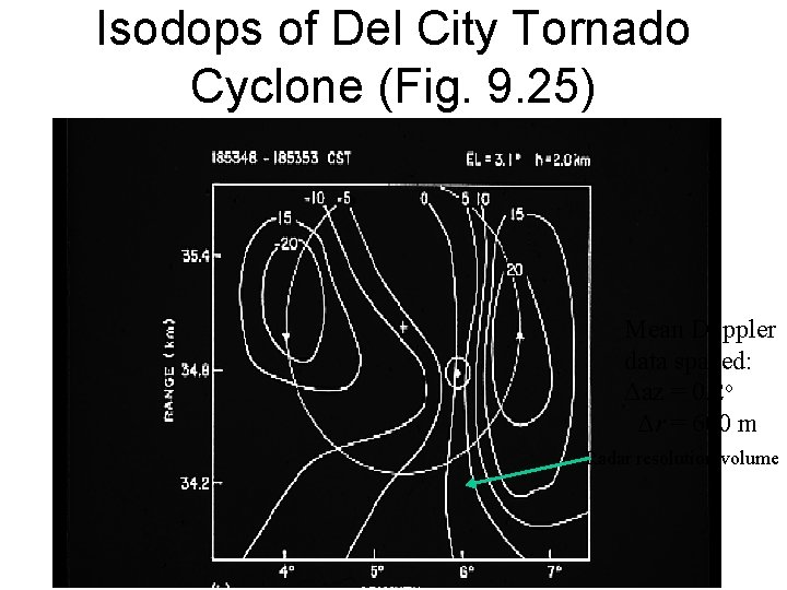
Isodops of Del City Tornado Cyclone (Fig. 9. 25) Mean Doppler data spaced: Δaz = 0. 2 o Δr = 600 m Radar resolution volume

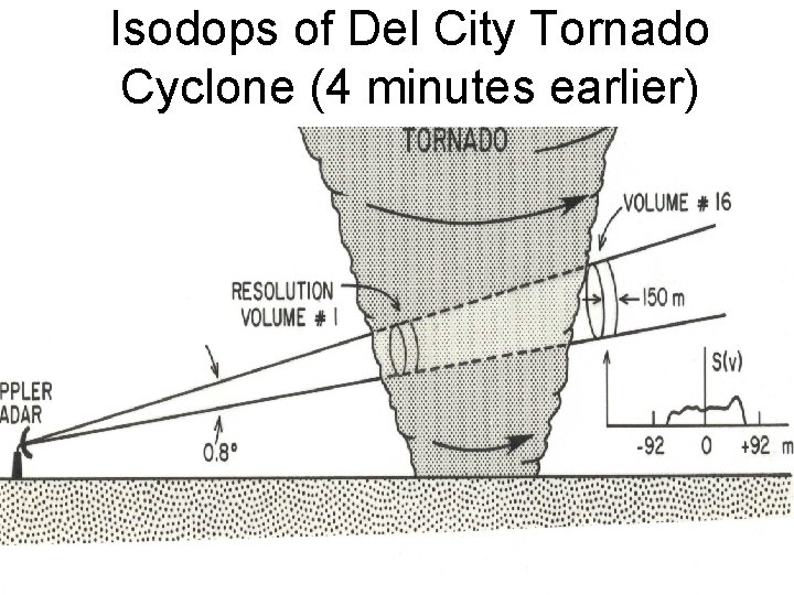
Isodops of Del City Tornado Cyclone (4 minutes earlier)

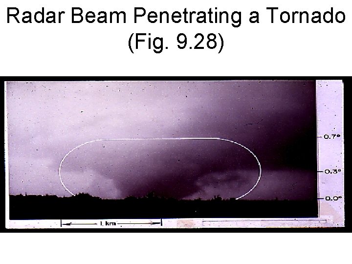
Radar Beam Penetrating a Tornado (Fig. 9. 28)

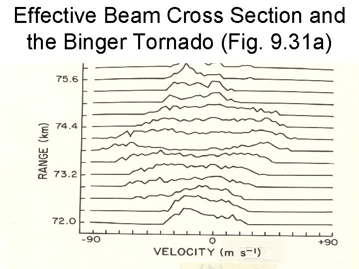
Effective Beam Cross Section and the Binger Tornado (Fig. 9. 31 a)

Binger Tornado Spectra (Fig. 9. 31 b)

Signal Processing to obtain accurate measurements of Doppler spectral moments and Polarimetric Variables (Chapter 6)

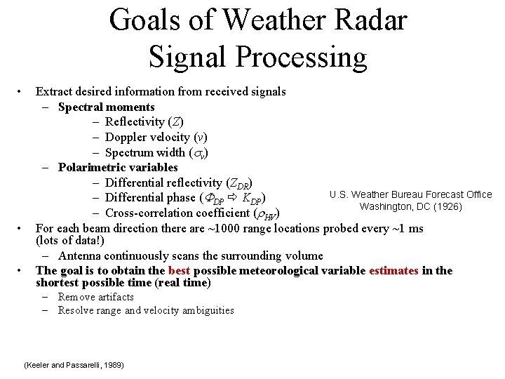
Goals of Weather Radar Signal Processing • • • Extract desired information from received signals – Spectral moments – Reflectivity (Z) – Doppler velocity (v) – Spectrum width (sv) – Polarimetric variables – Differential reflectivity (ZDR) U. S. Weather Bureau Forecast Office – Differential phase (FDP KDP) Washington, DC (1926) – Cross-correlation coefficient (r. HV) For each beam direction there are ~1000 range locations probed every ~1 ms (lots of data!) – Antenna continuously scans the surrounding volume The goal is to obtain the best possible meteorological variable estimates in the shortest possible time (real time) – Remove artifacts – Resolve range and velocity ambiguities (Keeler and Passarelli, 1989)

Chapter 6 deals mostly with statistical analysis of the variance of the estimates. Although variance of the estimates is important to the use of weather radar data, I have decided to skip any discussion of this topic. The bottom line of chapter 6: No matter how accurately we measure each weather signal echo sample, there is no way to make perfectly accurate measurements from a single echo sample! This so because weather echoes are random variables and measurements of one echo sample (e. g. , for power measurements), or a pair of samples (for Doppler measurements), has practically no meaning. Thus weather radar must process many echo samples and users of radar data must be content with estimates of the meteorological parameters of interest.