CHAPTER 14 MULTIPLE REGRESSION Prem Mann Introductory Statistics

CHAPTER 14 MULTIPLE REGRESSION Prem Mann, Introductory Statistics, 7/E Copyright © 2010 John Wiley & Sons. All right reserved

Opening Example Prem Mann, Introductory Statistics, 7/E Copyright © 2010 John Wiley & Sons. All right reserved

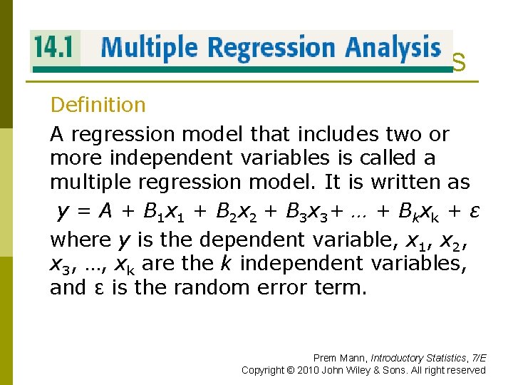
MULTIPLE REGRESSION ANALYSIS Definition A regression model that includes two or more independent variables is called a multiple regression model. It is written as y = A + B 1 x 1 + B 2 x 2 + B 3 x 3+ … + B kx k + ε where y is the dependent variable, x 1, x 2, x 3, …, xk are the k independent variables, and ε is the random error term. Prem Mann, Introductory Statistics, 7/E Copyright © 2010 John Wiley & Sons. All right reserved

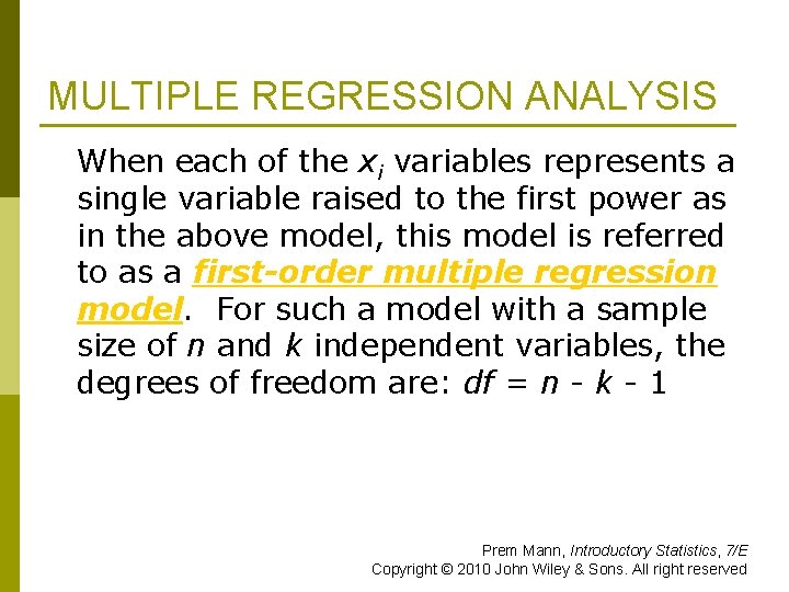
MULTIPLE REGRESSION ANALYSIS When each of the xi variables represents a single variable raised to the first power as in the above model, this model is referred to as a first-order multiple regression model. For such a model with a sample size of n and k independent variables, the degrees of freedom are: df = n - k - 1 Prem Mann, Introductory Statistics, 7/E Copyright © 2010 John Wiley & Sons. All right reserved

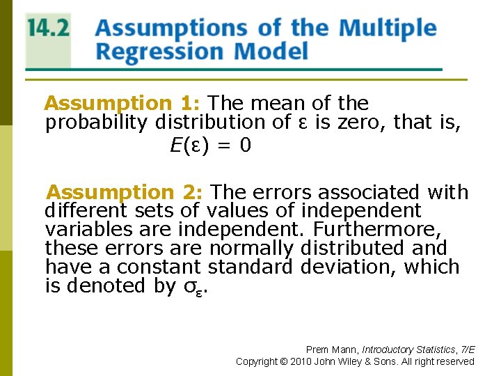
ASSUMPTIONS OF THE MULTIPLE REGRESSION MODEL Assumption 1: The mean of the probability distribution of ε is zero, that is, E(ε) = 0 Assumption 2: The errors associated with different sets of values of independent variables are independent. Furthermore, these errors are normally distributed and have a constant standard deviation, which is denoted by σε. Prem Mann, Introductory Statistics, 7/E Copyright © 2010 John Wiley & Sons. All right reserved

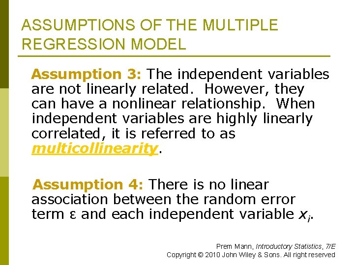
ASSUMPTIONS OF THE MULTIPLE REGRESSION MODEL Assumption 3: The independent variables are not linearly related. However, they can have a nonlinear relationship. When independent variables are highly linearly correlated, it is referred to as multicollinearity. Assumption 4: There is no linear association between the random error term ε and each independent variable xi. Prem Mann, Introductory Statistics, 7/E Copyright © 2010 John Wiley & Sons. All right reserved

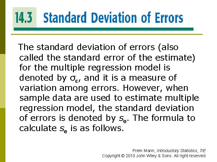
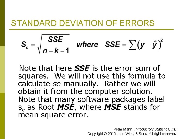
STANDARD DEVIATION OF ERRORS The standard deviation of errors (also called the standard error of the estimate) for the multiple regression model is denoted by σε, and it is a measure of variation among errors. However, when sample data are used to estimate multiple regression model, the standard deviation of errors is denoted by se. The formula to calculate se is as follows. Prem Mann, Introductory Statistics, 7/E Copyright © 2010 John Wiley & Sons. All right reserved

STANDARD DEVIATION OF ERRORS Note that here SSE is the error sum of squares. We will not use this formula to calculate se manually. Rather we will obtain it from the computer solution. Note that many software packages label se as Root MSE, where MSE stands for mean square error. Prem Mann, Introductory Statistics, 7/E Copyright © 2010 John Wiley & Sons. All right reserved

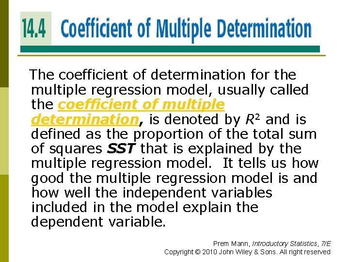
COEFFICIENT OF MULTIPLE DETERMINATION The coefficient of determination for the multiple regression model, usually called the coefficient of multiple determination, is denoted by R 2 and is defined as the proportion of the total sum of squares SST that is explained by the multiple regression model. It tells us how good the multiple regression model is and how well the independent variables included in the model explain the dependent variable. Prem Mann, Introductory Statistics, 7/E Copyright © 2010 John Wiley & Sons. All right reserved

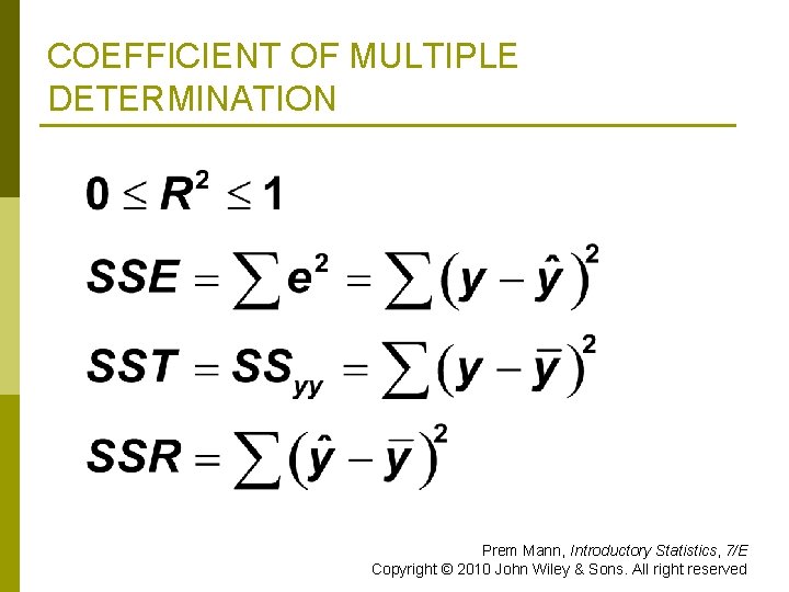
COEFFICIENT OF MULTIPLE DETERMINATION Prem Mann, Introductory Statistics, 7/E Copyright © 2010 John Wiley & Sons. All right reserved

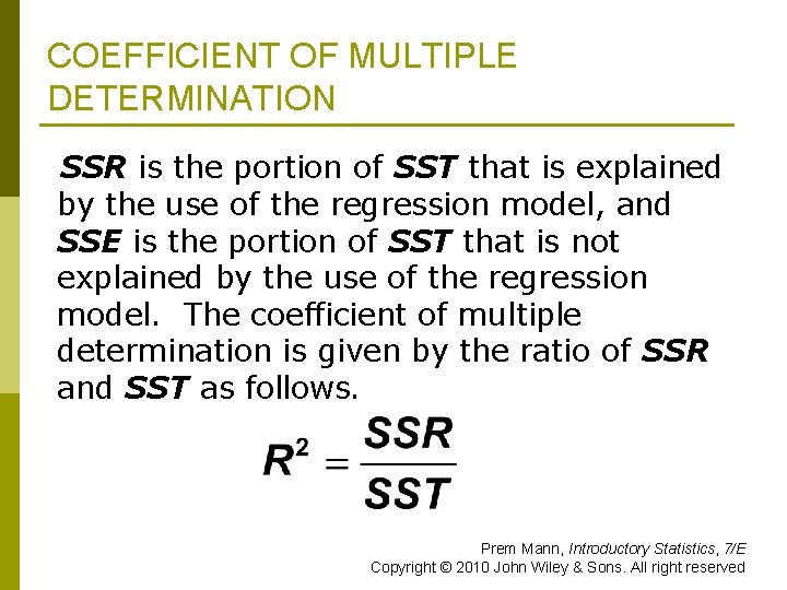
COEFFICIENT OF MULTIPLE DETERMINATION SSR is the portion of SST that is explained by the use of the regression model, and SSE is the portion of SST that is not explained by the use of the regression model. The coefficient of multiple determination is given by the ratio of SSR and SST as follows. Prem Mann, Introductory Statistics, 7/E Copyright © 2010 John Wiley & Sons. All right reserved

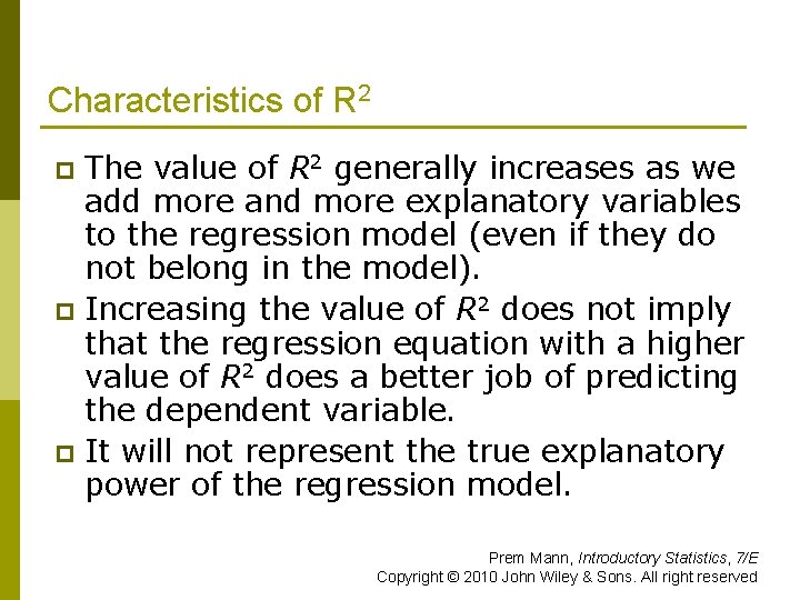
Characteristics of R 2 The value of R 2 generally increases as we add more and more explanatory variables to the regression model (even if they do not belong in the model). p Increasing the value of R 2 does not imply that the regression equation with a higher value of R 2 does a better job of predicting the dependent variable. p It will not represent the true explanatory power of the regression model. p Prem Mann, Introductory Statistics, 7/E Copyright © 2010 John Wiley & Sons. All right reserved

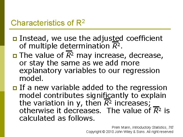
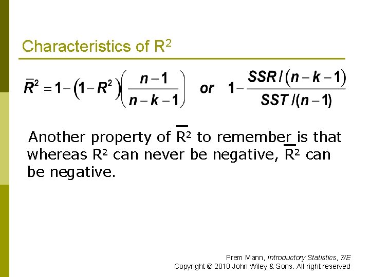
Characteristics of R 2 Instead, we use the adjusted coefficient of multiple determination R 2. p The value of R 2 may increase, decrease, or stay the same as we add more explanatory variables to our regression model. p If a new variable added to the regression model contributes significantly to explain the variation in y, then R 2 increases; otherwise it decreases. The value of R 2 is calculated as follows. p Prem Mann, Introductory Statistics, 7/E Copyright © 2010 John Wiley & Sons. All right reserved

Characteristics of R 2 Another property of R 2 to remember is that whereas R 2 can never be negative, R 2 can be negative. Prem Mann, Introductory Statistics, 7/E Copyright © 2010 John Wiley & Sons. All right reserved

COMPUTER SOLUTION OF MULTIPLE REGRESSION In this section, we take an example of a multiple regression model, solve it using MINITAB, interpret the solution, and make inferences about the population parameters of the regression model. Prem Mann, Introductory Statistics, 7/E Copyright © 2010 John Wiley & Sons. All right reserved

Example 14 -1 A researcher wanted to find the effect of driving experience and the number of driving violations on auto insurance premiums. A random sample of 12 drivers insured with the same company and having similar auto insurance policies was selected from a large city. Prem Mann, Introductory Statistics, 7/E Copyright © 2010 John Wiley & Sons. All right reserved

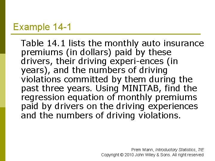
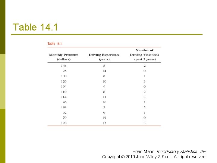
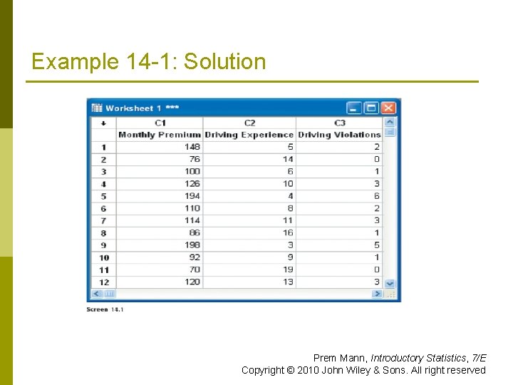
Example 14 -1 Table 14. 1 lists the monthly auto insurance premiums (in dollars) paid by these drivers, their driving experi ences (in years), and the numbers of driving violations committed by them during the past three years. Using MINITAB, find the regression equation of monthly premiums paid by drivers on the driving experiences and the numbers of driving violations. Prem Mann, Introductory Statistics, 7/E Copyright © 2010 John Wiley & Sons. All right reserved

Table 14. 1 Prem Mann, Introductory Statistics, 7/E Copyright © 2010 John Wiley & Sons. All right reserved

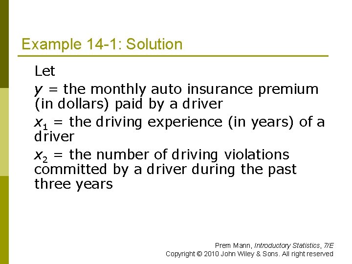
Example 14 -1: Solution Let y = the monthly auto insurance premium (in dollars) paid by a driver x 1 = the driving experience (in years) of a driver x 2 = the number of driving violations committed by a driver during the past three years Prem Mann, Introductory Statistics, 7/E Copyright © 2010 John Wiley & Sons. All right reserved

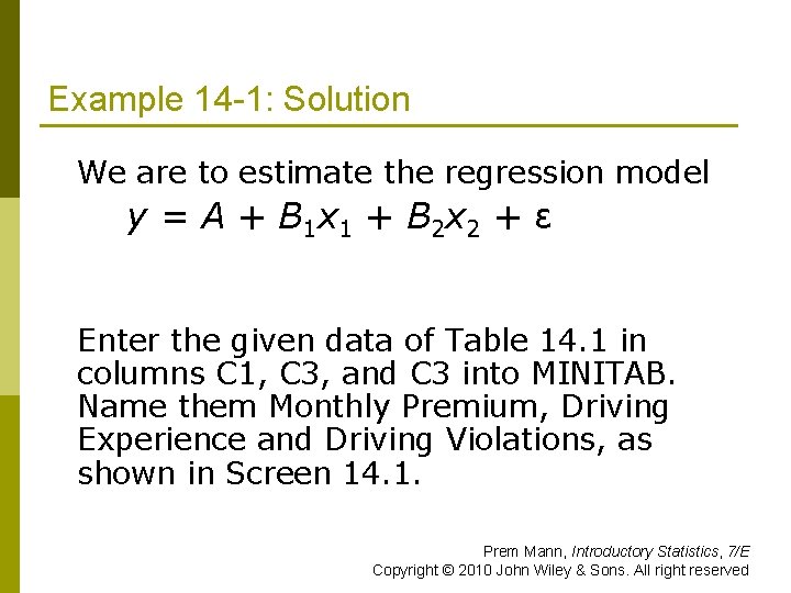
Example 14 -1: Solution We are to estimate the regression model y = A + B 1 x 1 + B 2 x 2 + ε Enter the given data of Table 14. 1 in columns C 1, C 3, and C 3 into MINITAB. Name them Monthly Premium, Driving Experience and Driving Violations, as shown in Screen 14. 1. Prem Mann, Introductory Statistics, 7/E Copyright © 2010 John Wiley & Sons. All right reserved

Example 14 -1: Solution. Prem Mann, Introductory Statistics, 7/E Copyright © 2010 John Wiley & Sons. All right reserved

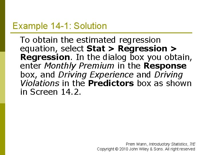
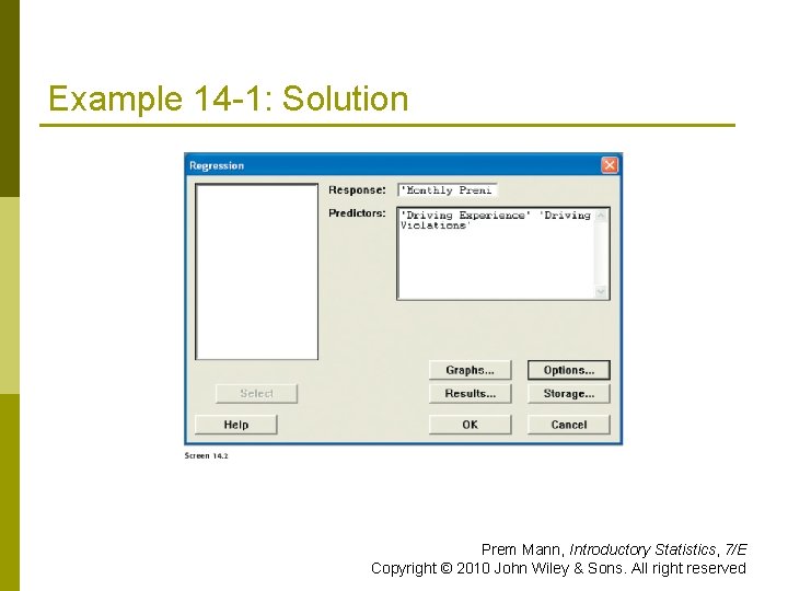
Example 14 -1: Solution To obtain the estimated regression equation, select Stat > Regression. In the dialog box you obtain, enter Monthly Premium in the Response box, and Driving Experience and Driving Violations in the Predictors box as shown in Screen 14. 2. Prem Mann, Introductory Statistics, 7/E Copyright © 2010 John Wiley & Sons. All right reserved

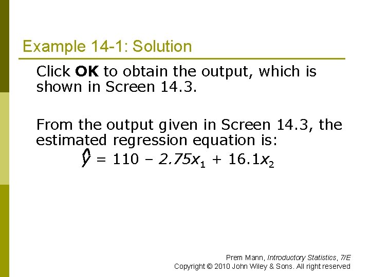
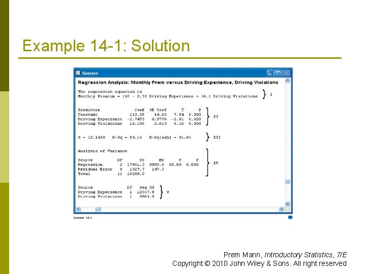
Example 14 -1: Solution Click OK to obtain the output, which is shown in Screen 14. 3. From the output given in Screen 14. 3, the estimated regression equation is: y = 110 – 2. 75 x 1 + 16. 1 x 2 Prem Mann, Introductory Statistics, 7/E Copyright © 2010 John Wiley & Sons. All right reserved

Example 14 -1: Solution Prem Mann, Introductory Statistics, 7/E Copyright © 2010 John Wiley & Sons. All right reserved

Example 14 -1: Solution Prem Mann, Introductory Statistics, 7/E Copyright © 2010 John Wiley & Sons. All right reserved

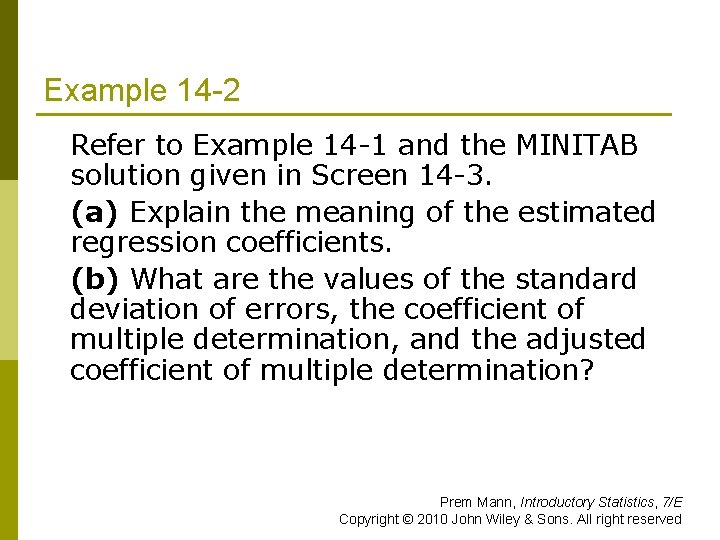
Example 14 -2 Refer to Example 14 1 and the MINITAB solution given in Screen 14 3. (a) Explain the meaning of the estimated regression coefficients. (b) What are the values of the standard deviation of errors, the coefficient of multiple determination, and the adjusted coefficient of multiple determination? Prem Mann, Introductory Statistics, 7/E Copyright © 2010 John Wiley & Sons. All right reserved

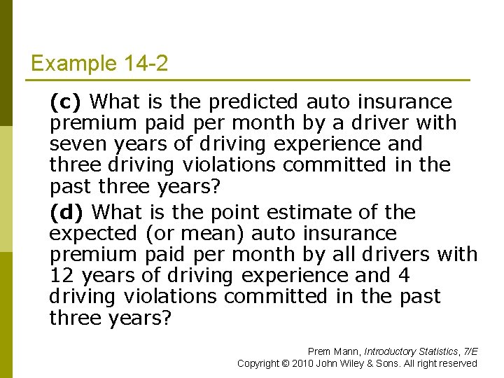
Example 14 -2 (c) What is the predicted auto insurance premium paid per month by a driver with seven years of driving experience and three driving violations committed in the past three years? (d) What is the point estimate of the expected (or mean) auto insurance premium paid per month by all drivers with 12 years of driving experience and 4 driving violations committed in the past three years? Prem Mann, Introductory Statistics, 7/E Copyright © 2010 John Wiley & Sons. All right reserved

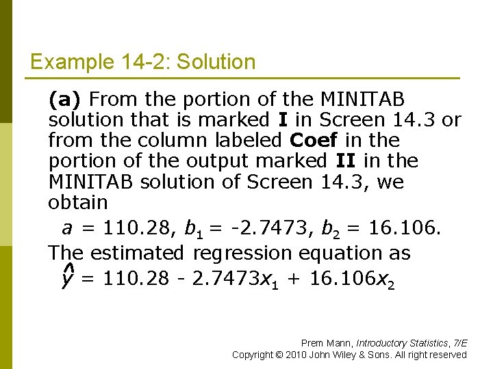
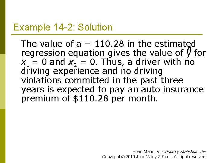
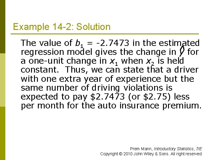
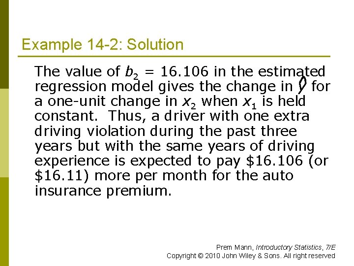
Example 14 -2: Solution (a) From the portion of the MINITAB solution that is marked I in Screen 14. 3 or from the column labeled Coef in the portion of the output marked II in the MINITAB solution of Screen 14. 3, we obtain a = 110. 28, b 1 = 2. 7473, b 2 = 16. 106. The estimated regression equation as y = 110. 28 2. 7473 x 1 + 16. 106 x 2 Prem Mann, Introductory Statistics, 7/E Copyright © 2010 John Wiley & Sons. All right reserved

Example 14 -2: Solution The value of a = 110. 28 in the estimated regression equation gives the value of y for x 1 = 0 and x 2 = 0. Thus, a driver with no driving experience and no driving violations committed in the past three years is expected to pay an auto insurance premium of $110. 28 per month. Prem Mann, Introductory Statistics, 7/E Copyright © 2010 John Wiley & Sons. All right reserved

Example 14 -2: Solution The value of b 1 = 2. 7473 in the estimated regression model gives the change in y for a one unit change in x 1 when x 2 is held constant. Thus, we can state that a driver with one extra year of experience but the same number of driving violations is expected to pay $2. 7473 (or $2. 75) less per month for the auto insurance premium. Prem Mann, Introductory Statistics, 7/E Copyright © 2010 John Wiley & Sons. All right reserved

Example 14 -2: Solution The value of b 2 = 16. 106 in the estimated regression model gives the change in y for a one unit change in x 2 when x 1 is held constant. Thus, a driver with one extra driving violation during the past three years but with the same years of driving experience is expected to pay $16. 106 (or $16. 11) more per month for the auto insurance premium. Prem Mann, Introductory Statistics, 7/E Copyright © 2010 John Wiley & Sons. All right reserved

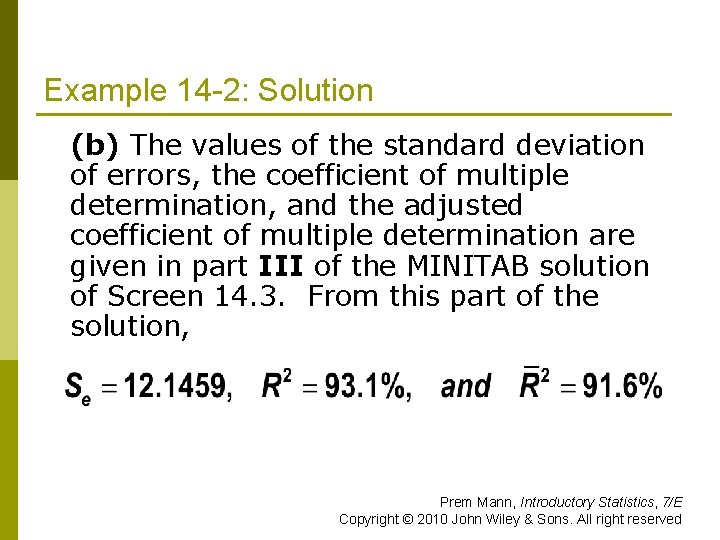
Example 14 -2: Solution (b) The values of the standard deviation of errors, the coefficient of multiple determination, and the adjusted coefficient of multiple determination are given in part III of the MINITAB solution of Screen 14. 3. From this part of the solution, Prem Mann, Introductory Statistics, 7/E Copyright © 2010 John Wiley & Sons. All right reserved

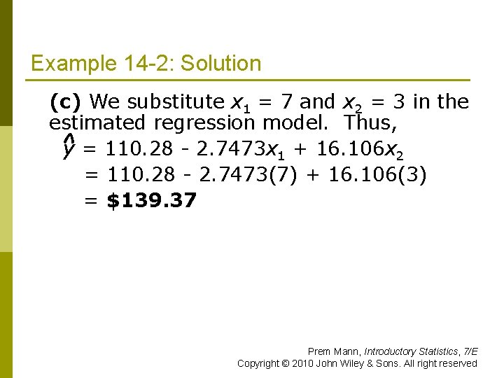
Example 14 -2: Solution (c) We substitute x 1 = 7 and x 2 = 3 in the estimated regression model. Thus, y = 110. 28 2. 7473 x 1 + 16. 106 x 2 = 110. 28 2. 7473(7) + 16. 106(3) = $139. 37 Prem Mann, Introductory Statistics, 7/E Copyright © 2010 John Wiley & Sons. All right reserved

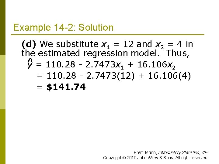
Example 14 -2: Solution (d) We substitute x 1 = 12 and x 2 = 4 in the estimated regression model. Thus, y = 110. 28 2. 7473 x 1 + 16. 106 x 2 = 110. 28 2. 7473(12) + 16. 106(4) = $141. 74 Prem Mann, Introductory Statistics, 7/E Copyright © 2010 John Wiley & Sons. All right reserved

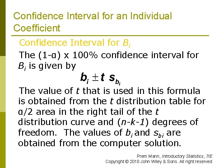
Confidence Interval for an Individual Coefficient Confidence Interval for Bi The (1 α) x 100% confidence interval for Bi is given by The value of t that is used in this formula is obtained from the t distribution table for α/2 area in the right tail of the t distribution curve and (n-k-1) degrees of freedom. The values of bi and sbi are obtained from the computer solution. Prem Mann, Introductory Statistics, 7/E Copyright © 2010 John Wiley & Sons. All right reserved

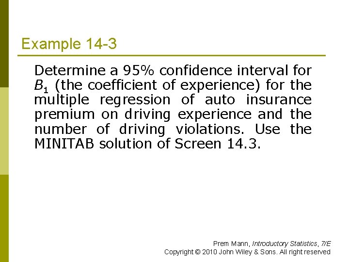
Example 14 -3 Determine a 95% confidence interval for B 1 (the coefficient of experience) for the multiple regression of auto insurance premium on driving experience and the number of driving violations. Use the MINITAB solution of Screen 14. 3. Prem Mann, Introductory Statistics, 7/E Copyright © 2010 John Wiley & Sons. All right reserved

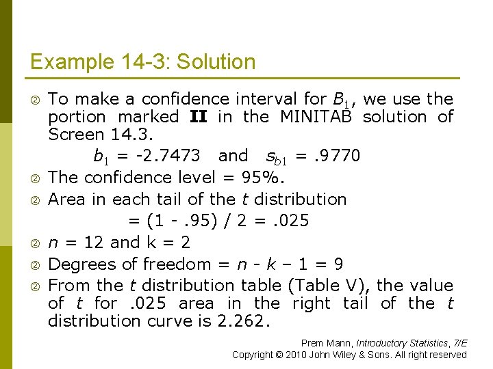
Example 14 -3: Solution To make a confidence interval for B 1, we use the portion marked II in the MINITAB solution of Screen 14. 3. b 1 = 2. 7473 and sb 1 =. 9770 The confidence level = 95%. Area in each tail of the t distribution = (1 . 95) / 2 =. 025 n = 12 and k = 2 Degrees of freedom = n - k – 1 = 9 From the t distribution table (Table V), the value of t for. 025 area in the right tail of the t distribution curve is 2. 262. Prem Mann, Introductory Statistics, 7/E Copyright © 2010 John Wiley & Sons. All right reserved

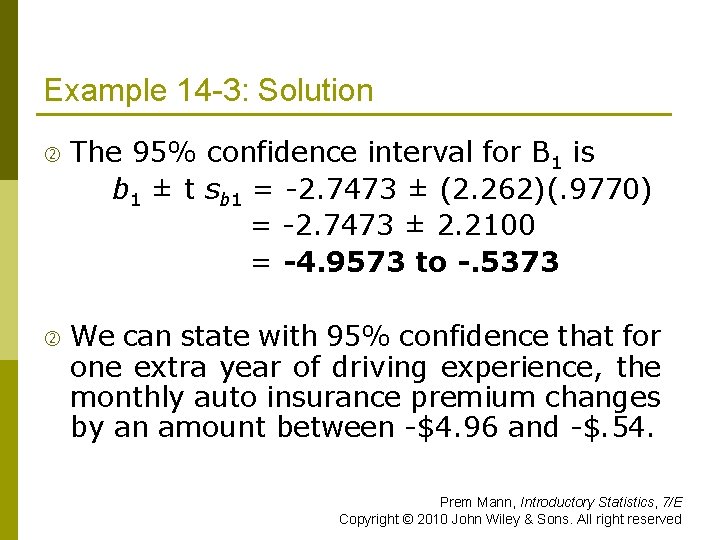
Example 14 -3: Solution The 95% confidence interval for B 1 is b 1 ± t sb 1 = 2. 7473 ± (2. 262)(. 9770) = 2. 7473 ± 2. 2100 = -4. 9573 to -. 5373 We can state with 95% confidence that for one extra year of driving experience, the monthly auto insurance premium changes by an amount between $4. 96 and $. 54. Prem Mann, Introductory Statistics, 7/E Copyright © 2010 John Wiley & Sons. All right reserved

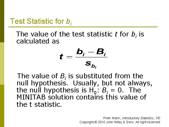
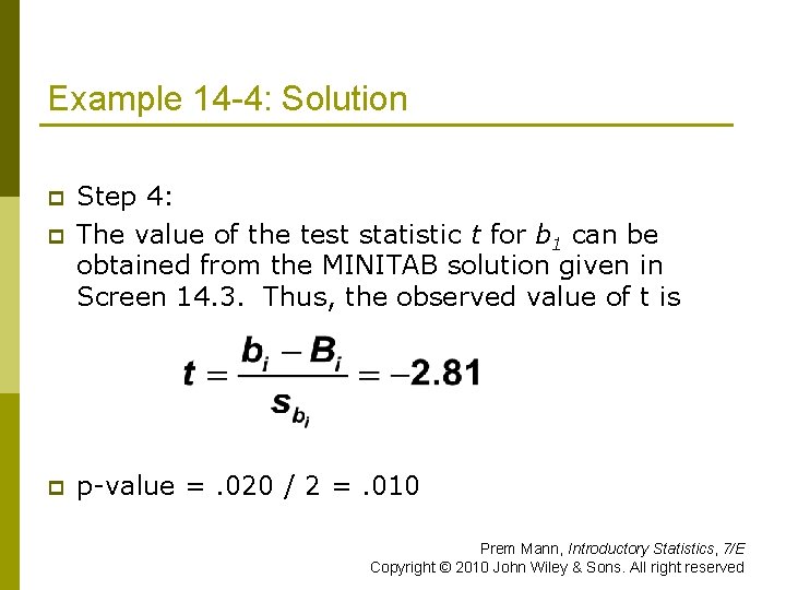
Test Statistic for bi The value of the test statistic t for bi is calculated as The value of Bi is substituted from the null hypothesis. Usually, but not always, the null hypothesis is H 0: Bi = 0. The MINITAB solution contains this value of the t statistic. Prem Mann, Introductory Statistics, 7/E Copyright © 2010 John Wiley & Sons. All right reserved

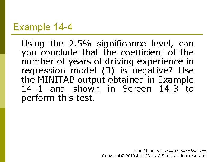
Example 14 -4 Using the 2. 5% significance level, can you conclude that the coefficient of the number of years of driving experience in regression model (3) is negative? Use the MINITAB output obtained in Example 14– 1 and shown in Screen 14. 3 to perform this test. Prem Mann, Introductory Statistics, 7/E Copyright © 2010 John Wiley & Sons. All right reserved

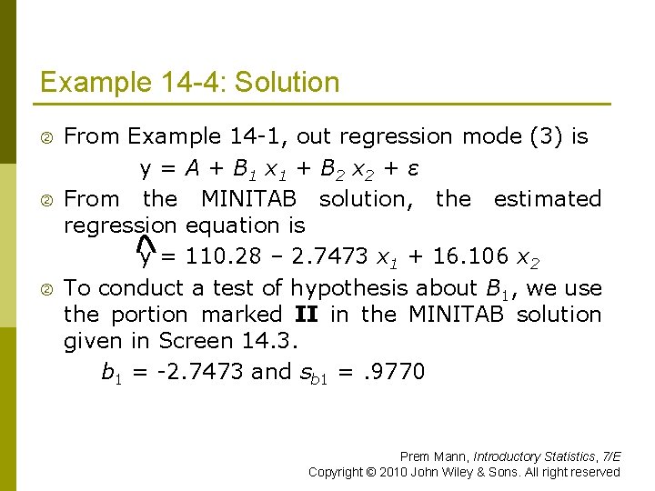
Example 14 -4: Solution From Example 14 1, out regression mode (3) is y = A + B 1 x 1 + B 2 x 2 + ε From the MINITAB solution, the estimated regression equation is y = 110. 28 – 2. 7473 x 1 + 16. 106 x 2 To conduct a test of hypothesis about B 1, we use the portion marked II in the MINITAB solution given in Screen 14. 3. b 1 = 2. 7473 and sb 1 =. 9770 Prem Mann, Introductory Statistics, 7/E Copyright © 2010 John Wiley & Sons. All right reserved

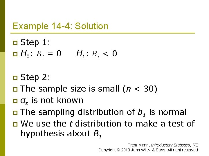
Example 14 -4: Solution Step 1: p H 0: B 1 = 0 p H 1: B 1 < 0 Step 2: p The sample size is small (n < 30) p σε is not known p The sampling distribution of b 1 is normal p We use the t distribution to make a test of hypothesis about B 1 p Prem Mann, Introductory Statistics, 7/E Copyright © 2010 John Wiley & Sons. All right reserved

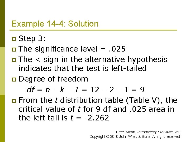
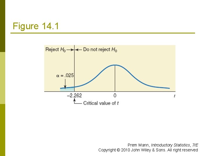
Example 14 -4: Solution Step 3: p The significance level =. 025 p The < sign in the alternative hypothesis indicates that the test is left tailed p Degree of freedom df = n – k – 1 = 12 – 1 = 9 p From the t distribution table (Table V), the critical value of t for 9 df and. 025 area in the left tail is t = 2. 262 p Prem Mann, Introductory Statistics, 7/E Copyright © 2010 John Wiley & Sons. All right reserved

Figure 14. 1 Prem Mann, Introductory Statistics, 7/E Copyright © 2010 John Wiley & Sons. All right reserved

Example 14 -4: Solution p Step 4: The value of the test statistic t for b 1 can be obtained from the MINITAB solution given in Screen 14. 3. Thus, the observed value of t is p p value =. 020 / 2 =. 010 p Prem Mann, Introductory Statistics, 7/E Copyright © 2010 John Wiley & Sons. All right reserved

Example 14 -4: Solution Step 5: p The value of the test statistic t = 2. 81 p It is less than the critical value t = 2. 262 p If falls in the rejection region p We reject the null hypothesis p We conclude that the coefficient of x 1 in regression mode (3) is negative. p Prem Mann, Introductory Statistics, 7/E Copyright © 2010 John Wiley & Sons. All right reserved