CHAPTER 12 CHISQUARE TESTS Prem Mann Introductory Statistics

CHAPTER 12 CHI-SQUARE TESTS Prem Mann, Introductory Statistics, 7/E Copyright © 2010 John Wiley & Sons. All right reserved

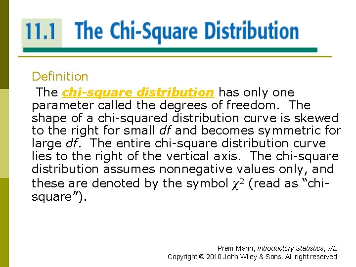
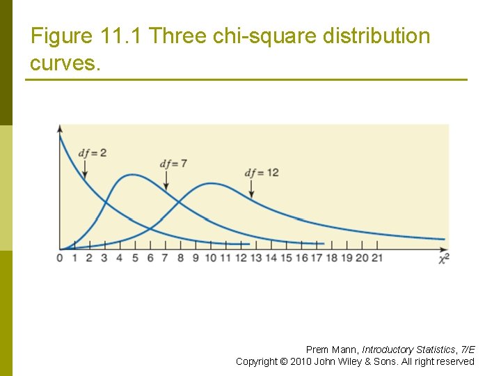
THE CHI-SQUARE DISTRIBUTION Definition The chi-square distribution has only one parameter called the degrees of freedom. The shape of a chi-squared distribution curve is skewed to the right for small df and becomes symmetric for large df. The entire chi-square distribution curve lies to the right of the vertical axis. The chi-square distribution assumes nonnegative values only, and these are denoted by the symbol χ2 (read as “chisquare”). Prem Mann, Introductory Statistics, 7/E Copyright © 2010 John Wiley & Sons. All right reserved

Figure 11. 1 Three chi-square distribution curves. Prem Mann, Introductory Statistics, 7/E Copyright © 2010 John Wiley & Sons. All right reserved

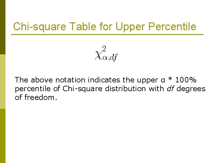
Chi-square Table for Upper Percentile The above notation indicates the upper α * 100% percentile of Chi-square distribution with df degrees of freedom.

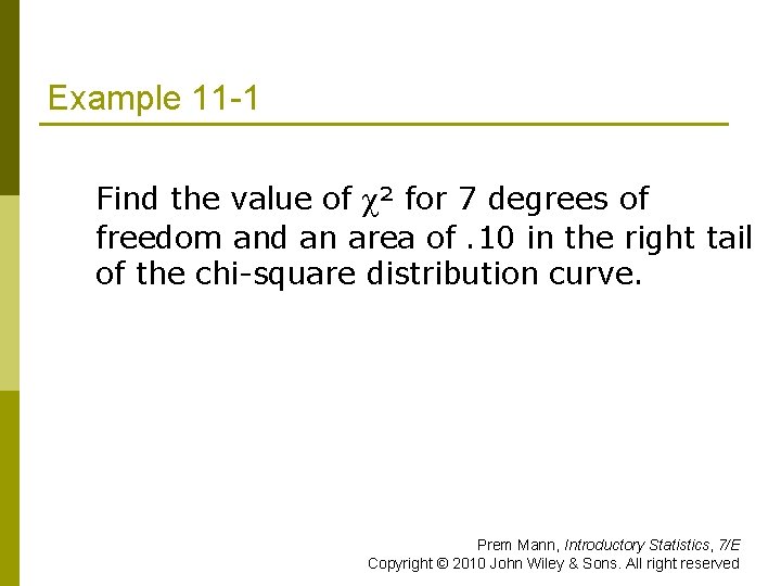
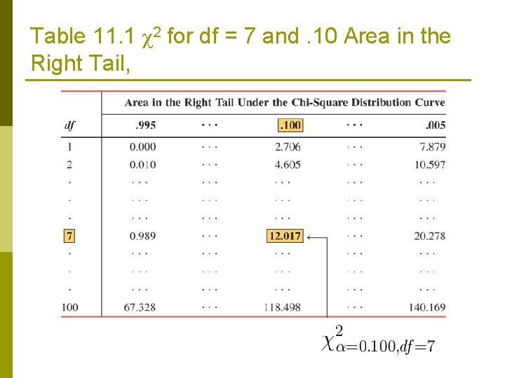
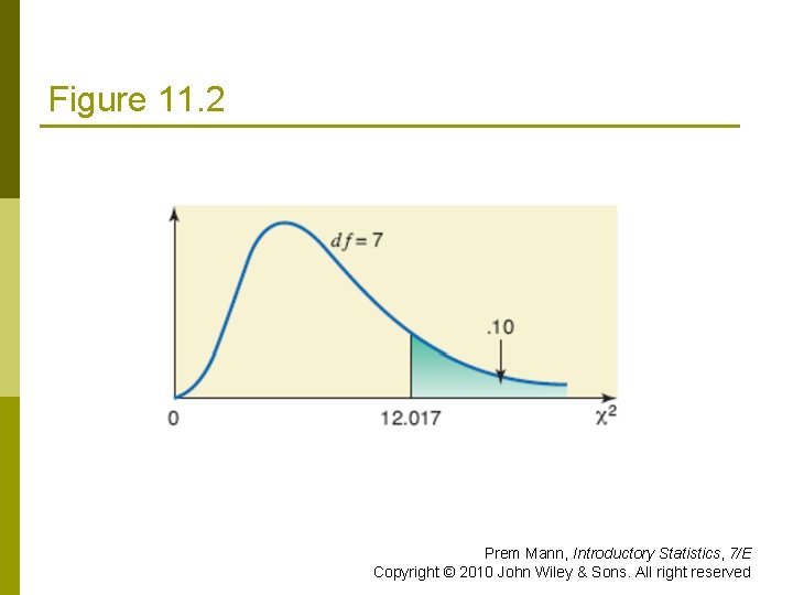
Example 11 -1 Find the value of χ² for 7 degrees of freedom and an area of. 10 in the right tail of the chi-square distribution curve. Prem Mann, Introductory Statistics, 7/E Copyright © 2010 John Wiley & Sons. All right reserved

Table 11. 1 χ2 for df = 7 and. 10 Area in the Right Tail,

Figure 11. 2 Prem Mann, Introductory Statistics, 7/E Copyright © 2010 John Wiley & Sons. All right reserved

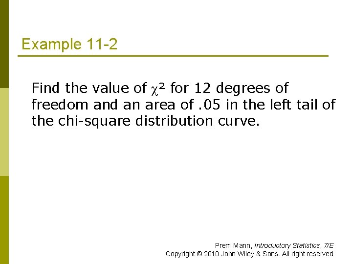
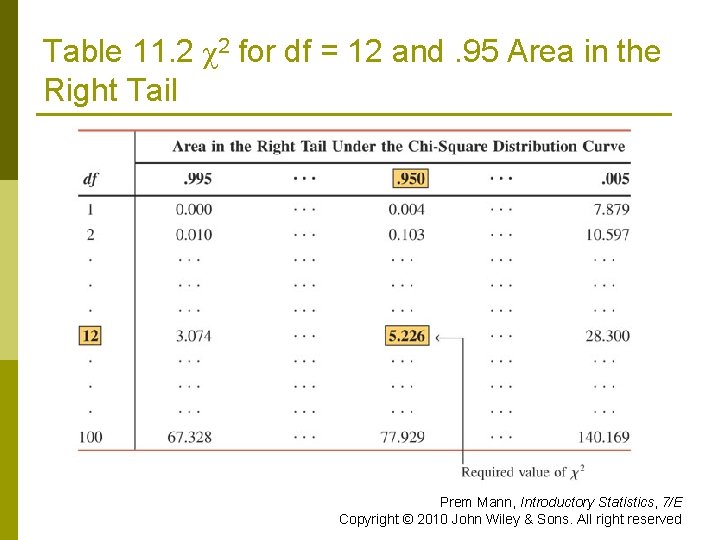
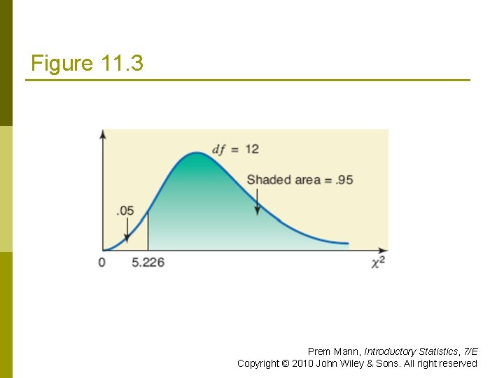
Example 11 -2 Find the value of χ² for 12 degrees of freedom and an area of. 05 in the left tail of the chi-square distribution curve. Prem Mann, Introductory Statistics, 7/E Copyright © 2010 John Wiley & Sons. All right reserved

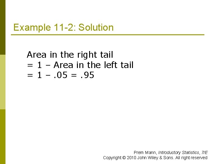
Example 11 -2: Solution Area in the right tail = 1 – Area in the left tail = 1 –. 05 =. 95 Prem Mann, Introductory Statistics, 7/E Copyright © 2010 John Wiley & Sons. All right reserved

Table 11. 2 χ2 for df = 12 and. 95 Area in the Right Tail Prem Mann, Introductory Statistics, 7/E Copyright © 2010 John Wiley & Sons. All right reserved

Figure 11. 3 Prem Mann, Introductory Statistics, 7/E Copyright © 2010 John Wiley & Sons. All right reserved

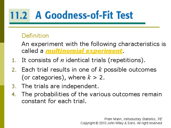
A GOODNESS-OF-FIT TEST Definition An experiment with the following characteristics is called a multinomial experiment. 1. It consists of n identical trials (repetitions). 2. Each trial results in one of k possible outcomes (or categories), where k > 2. The trials are independent. 4. The probabilities of the various outcomes remain constant for each trial. 3. Prem Mann, Introductory Statistics, 7/E Copyright © 2010 John Wiley & Sons. All right reserved

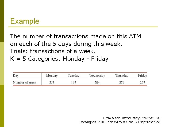
Example The number of transactions made on this ATM on each of the 5 days during this week. Trials: transactions of a week. K = 5 Categories: Monday - Friday Prem Mann, Introductory Statistics, 7/E Copyright © 2010 John Wiley & Sons. All right reserved

A GOODNESS-OF-FIT TEST Definition The frequencies obtained from the performance of an experiment are called the observed frequencies and are denoted by O. The expected frequencies, denoted by E, are the frequencies that we expect to obtain if the null hypothesis is true. The expected frequency for a category is obtained as E = np where n is the sample size and p is the probability that an element belongs to that category if the null hypothesis is true. Prem Mann, Introductory Statistics, 7/E Copyright © 2010 John Wiley & Sons. All right reserved

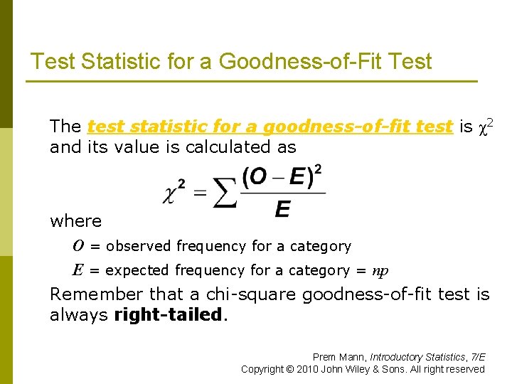
Test Statistic for a Goodness-of-Fit Test The test statistic for a goodness-of-fit test is χ2 and its value is calculated as where O = observed frequency for a category E = expected frequency for a category = np Remember that a chi-square goodness-of-fit test is always right-tailed. Prem Mann, Introductory Statistics, 7/E Copyright © 2010 John Wiley & Sons. All right reserved

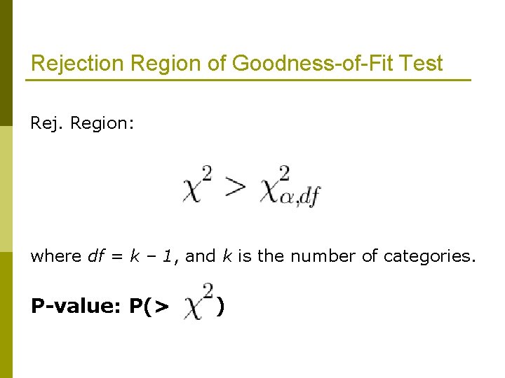
Rejection Region of Goodness-of-Fit Test Rej. Region: where df = k – 1, and k is the number of categories. P-value: P(> )

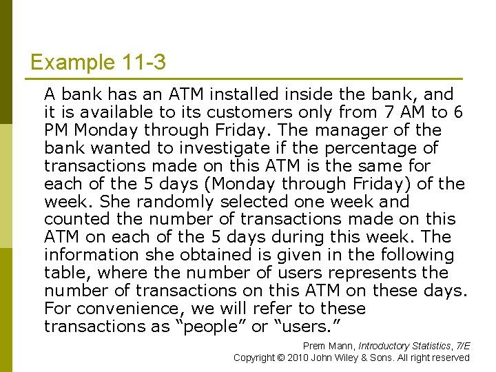
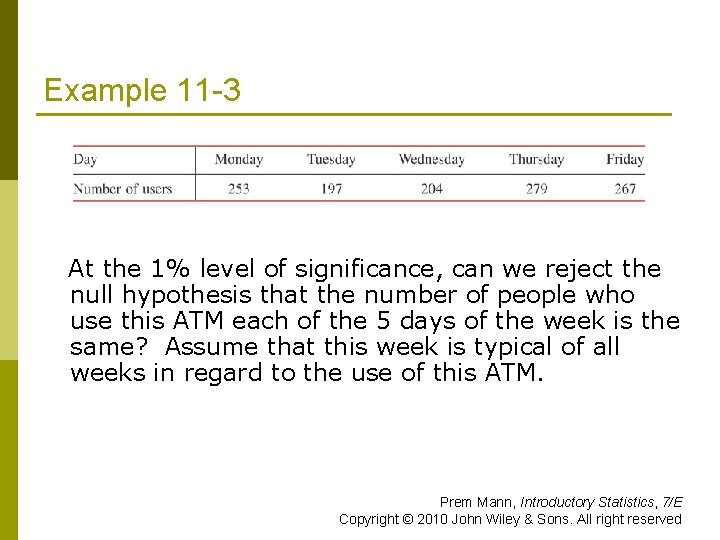
Example 11 -3 A bank has an ATM installed inside the bank, and it is available to its customers only from 7 AM to 6 PM Monday through Friday. The manager of the bank wanted to investigate if the percentage of transactions made on this ATM is the same for each of the 5 days (Monday through Friday) of the week. She randomly selected one week and counted the number of transactions made on this ATM on each of the 5 days during this week. The information she obtained is given in the following table, where the number of users represents the number of transactions on this ATM on these days. For convenience, we will refer to these transactions as “people” or “users. ” Prem Mann, Introductory Statistics, 7/E Copyright © 2010 John Wiley & Sons. All right reserved

Example 11 -3 At the 1% level of significance, can we reject the null hypothesis that the number of people who use this ATM each of the 5 days of the week is the same? Assume that this week is typical of all weeks in regard to the use of this ATM. Prem Mann, Introductory Statistics, 7/E Copyright © 2010 John Wiley & Sons. All right reserved

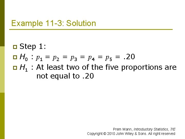
Example 11 -3: Solution Step 1: p H 0 : p 1 = p 2 = p 3 = p 4 = p 5 =. 20 p H 1 : At least two of the five proportions are not equal to. 20 p Prem Mann, Introductory Statistics, 7/E Copyright © 2010 John Wiley & Sons. All right reserved

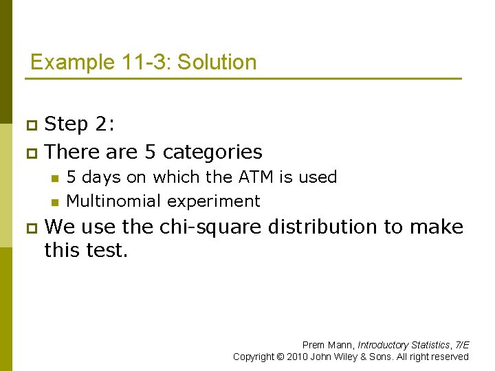
Example 11 -3: Solution Step 2: p There are 5 categories p n n p 5 days on which the ATM is used Multinomial experiment We use the chi-square distribution to make this test. Prem Mann, Introductory Statistics, 7/E Copyright © 2010 John Wiley & Sons. All right reserved

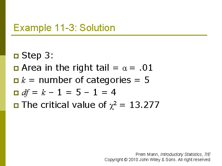
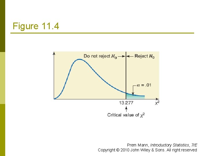
Example 11 -3: Solution Step 3: p Area in the right tail = α =. 01 p k = number of categories = 5 p df = k – 1 = 5 – 1 = 4 p The critical value of χ2 = 13. 277 p Prem Mann, Introductory Statistics, 7/E Copyright © 2010 John Wiley & Sons. All right reserved

Figure 11. 4 Prem Mann, Introductory Statistics, 7/E Copyright © 2010 John Wiley & Sons. All right reserved

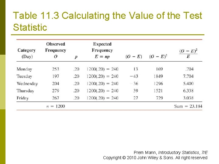
Table 11. 3 Calculating the Value of the Test Statistic Prem Mann, Introductory Statistics, 7/E Copyright © 2010 John Wiley & Sons. All right reserved

Example 11 -3: Solution Step 4: p All the required calculations to find the value of the test statistic χ2 are shown in Table 11. 3. p p Prem Mann, Introductory Statistics, 7/E Copyright © 2010 John Wiley & Sons. All right reserved

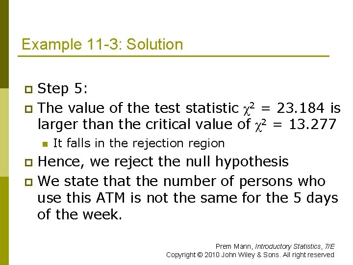
Example 11 -3: Solution Step 5: p The value of the test statistic χ2 = 23. 184 is larger than the critical value of χ2 = 13. 277 p n It falls in the rejection region Hence, we reject the null hypothesis p We state that the number of persons who use this ATM is not the same for the 5 days of the week. p Prem Mann, Introductory Statistics, 7/E Copyright © 2010 John Wiley & Sons. All right reserved

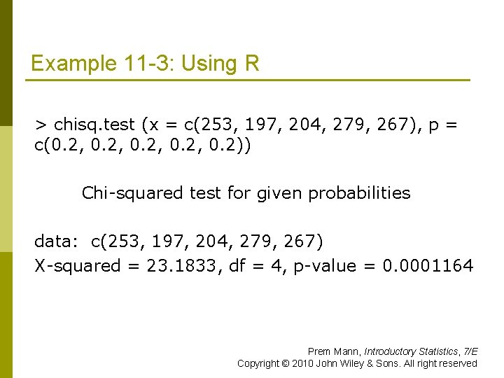
Example 11 -3: Using R > chisq. test (x = c(253, 197, 204, 279, 267), p = c(0. 2, 0. 2)) Chi-squared test for given probabilities data: c(253, 197, 204, 279, 267) X-squared = 23. 1833, df = 4, p-value = 0. 0001164 Prem Mann, Introductory Statistics, 7/E Copyright © 2010 John Wiley & Sons. All right reserved

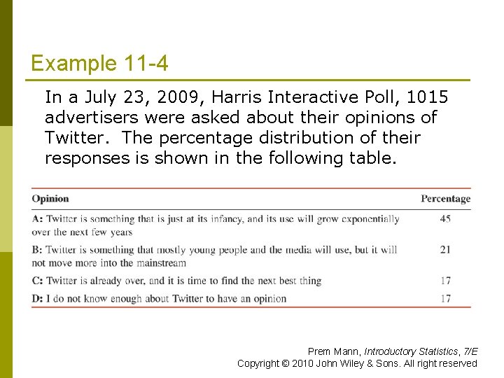
Example 11 -4 In a July 23, 2009, Harris Interactive Poll, 1015 advertisers were asked about their opinions of Twitter. The percentage distribution of their responses is shown in the following table. Prem Mann, Introductory Statistics, 7/E Copyright © 2010 John Wiley & Sons. All right reserved

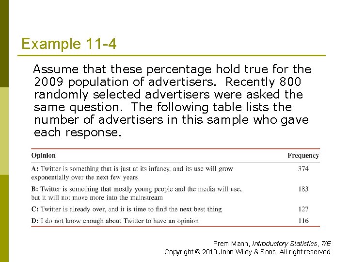
Example 11 -4 Assume that these percentage hold true for the 2009 population of advertisers. Recently 800 randomly selected advertisers were asked the same question. The following table lists the number of advertisers in this sample who gave each response. Prem Mann, Introductory Statistics, 7/E Copyright © 2010 John Wiley & Sons. All right reserved

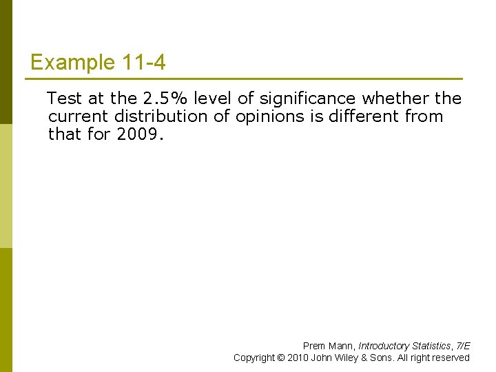
Example 11 -4 Test at the 2. 5% level of significance whether the current distribution of opinions is different from that for 2009. Prem Mann, Introductory Statistics, 7/E Copyright © 2010 John Wiley & Sons. All right reserved

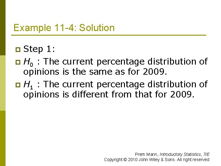
Example 11 -4: Solution Step 1: p H 0 : The opinions p H 1 : The opinions p current percentage distribution of is the same as for 2009. current percentage distribution of is different from that for 2009. Prem Mann, Introductory Statistics, 7/E Copyright © 2010 John Wiley & Sons. All right reserved

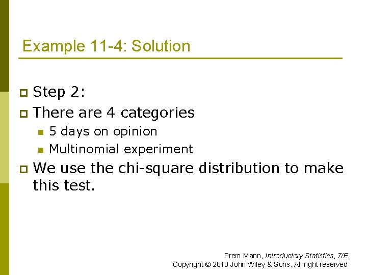
Example 11 -4: Solution Step 2: p There are 4 categories p n n p 5 days on opinion Multinomial experiment We use the chi-square distribution to make this test. Prem Mann, Introductory Statistics, 7/E Copyright © 2010 John Wiley & Sons. All right reserved

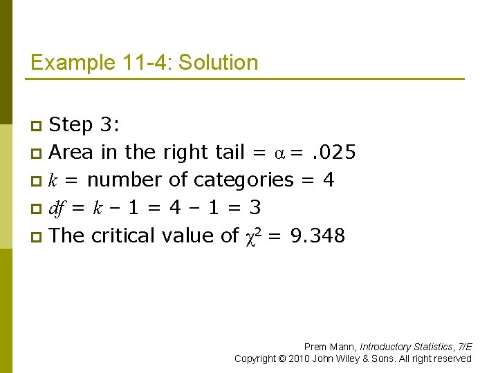
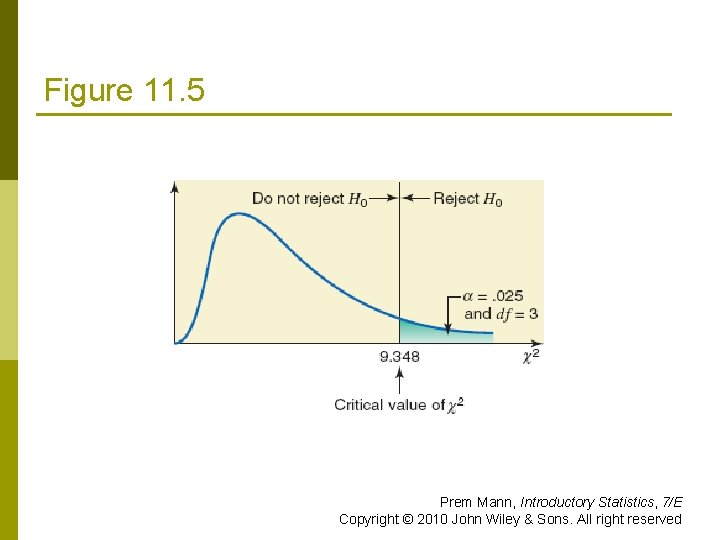
Example 11 -4: Solution Step 3: p Area in the right tail = α =. 025 p k = number of categories = 4 p df = k – 1 = 4 – 1 = 3 p The critical value of χ2 = 9. 348 p Prem Mann, Introductory Statistics, 7/E Copyright © 2010 John Wiley & Sons. All right reserved

Figure 11. 5 Prem Mann, Introductory Statistics, 7/E Copyright © 2010 John Wiley & Sons. All right reserved

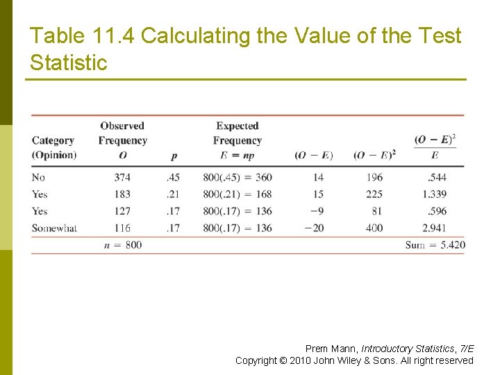
Table 11. 4 Calculating the Value of the Test Statistic Prem Mann, Introductory Statistics, 7/E Copyright © 2010 John Wiley & Sons. All right reserved

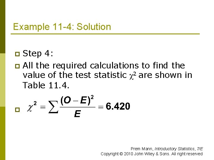
Example 11 -4: Solution Step 4: p All the required calculations to find the value of the test statistic χ2 are shown in Table 11. 4. p p Prem Mann, Introductory Statistics, 7/E Copyright © 2010 John Wiley & Sons. All right reserved

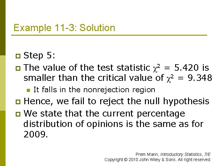
Example 11 -3: Solution Step 5: p The value of the test statistic χ2 = 5. 420 is smaller than the critical value of χ2 = 9. 348 p n It falls in the nonrejection region Hence, we fail to reject the null hypothesis p We state that the current percentage distribution of opinions is the same as for 2009. p Prem Mann, Introductory Statistics, 7/E Copyright © 2010 John Wiley & Sons. All right reserved

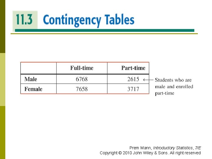
CONTINGENCY TABLES Prem Mann, Introductory Statistics, 7/E Copyright © 2010 John Wiley & Sons. All right reserved

A TEST OF INDEPENDENCE OR HOMOGENEITY A Test of Independence p A Test of Homogeneity p Prem Mann, Introductory Statistics, 7/E Copyright © 2010 John Wiley & Sons. All right reserved

A Test of Independence A test of independence involves a test of the null hypothesis that two attributes of a population are not related. Prem Mann, Introductory Statistics, 7/E Copyright © 2010 John Wiley & Sons. All right reserved

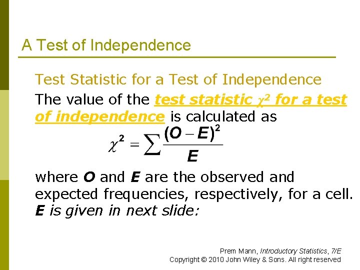
A Test of Independence Test Statistic for a Test of Independence The value of the test statistic χ2 for a test of independence is calculated as where O and E are the observed and expected frequencies, respectively, for a cell. E is given in next slide: Prem Mann, Introductory Statistics, 7/E Copyright © 2010 John Wiley & Sons. All right reserved

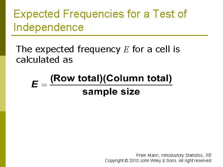
Expected Frequencies for a Test of Independence The expected frequency E for a cell is calculated as Prem Mann, Introductory Statistics, 7/E Copyright © 2010 John Wiley & Sons. All right reserved

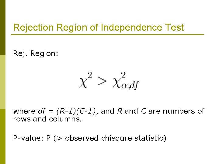
Rejection Region of Independence Test Rej. Region: where df = (R-1)(C-1), and R and C are numbers of rows and columns. P-value: P (> observed chisqure statistic)

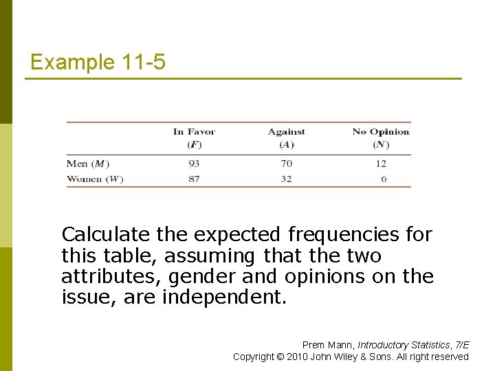
Example 11 -5 Violence and lack of discipline have become major problems in schools in the United States. A random sample of 300 adults was selected, and these adults were asked if they favor giving more freedom to schoolteachers to punish students for violence and lack of discipline. The two-way classification of the responses of these adults is represented in the following table. Prem Mann, Introductory Statistics, 7/E Copyright © 2010 John Wiley & Sons. All right reserved

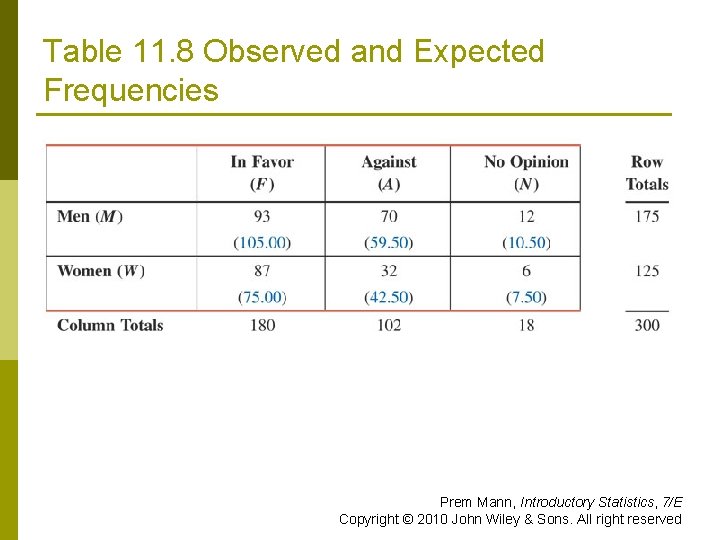
Example 11 -5 Calculate the expected frequencies for this table, assuming that the two attributes, gender and opinions on the issue, are independent. Prem Mann, Introductory Statistics, 7/E Copyright © 2010 John Wiley & Sons. All right reserved

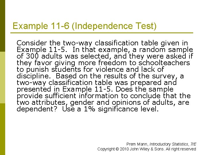
Example 11 -6 (Independence Test) Consider the two-way classification table given in Example 11 -5. In that example, a random sample of 300 adults was selected, and they were asked if they favor giving more freedom to schoolteachers to punish students for violence and lack of discipline. Based on the results of the survey, a two-way classification table was prepared and presented in Example 11 -5. Does the sample provide sufficient information to conclude that the two attributes, gender and opinions of adults, are dependent? Use a 1% significance level. Prem Mann, Introductory Statistics, 7/E Copyright © 2010 John Wiley & Sons. All right reserved

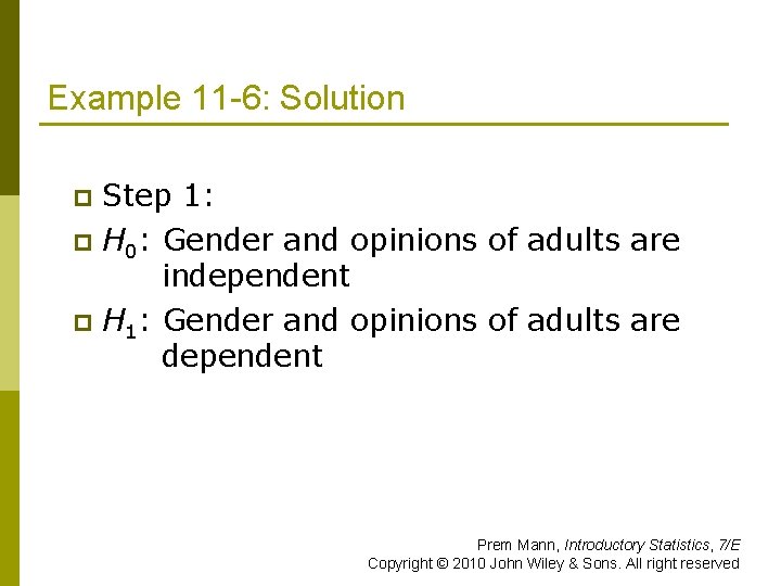
Example 11 -6: Solution Step 1: p H 0: Gender and opinions of adults are independent p H 1: Gender and opinions of adults are dependent p Prem Mann, Introductory Statistics, 7/E Copyright © 2010 John Wiley & Sons. All right reserved

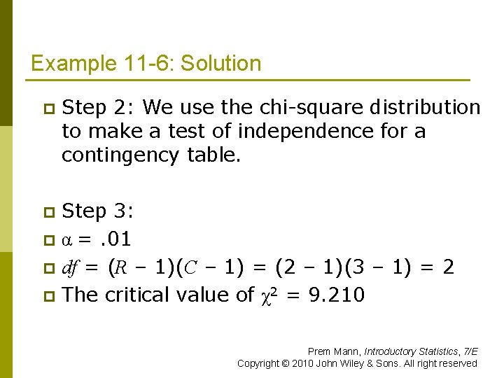
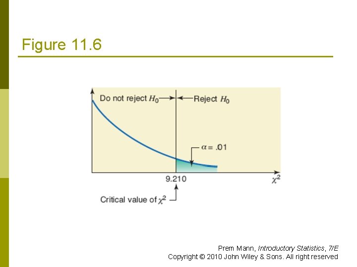
Example 11 -6: Solution p Step 2: We use the chi-square distribution to make a test of independence for a contingency table. Step 3: p α =. 01 p df = (R – 1)(C – 1) = (2 – 1)(3 – 1) = 2 p The critical value of χ2 = 9. 210 p Prem Mann, Introductory Statistics, 7/E Copyright © 2010 John Wiley & Sons. All right reserved

Figure 11. 6 Prem Mann, Introductory Statistics, 7/E Copyright © 2010 John Wiley & Sons. All right reserved

Table 11. 8 Observed and Expected Frequencies Prem Mann, Introductory Statistics, 7/E Copyright © 2010 John Wiley & Sons. All right reserved

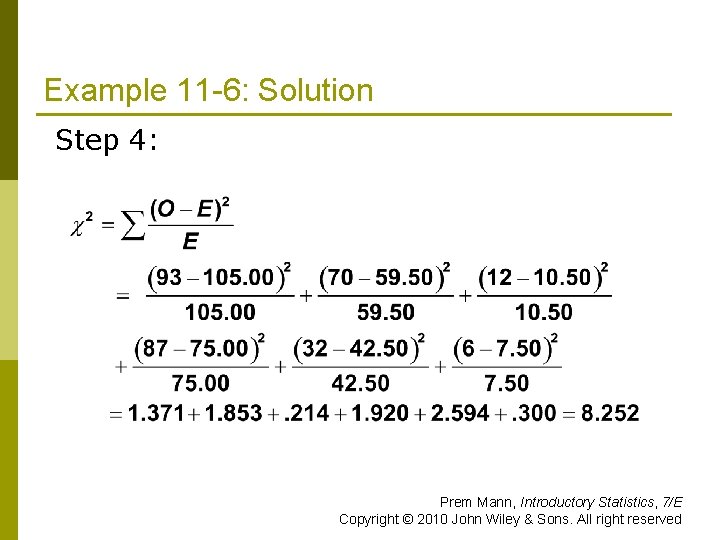
Example 11 -6: Solution Step 4: Prem Mann, Introductory Statistics, 7/E Copyright © 2010 John Wiley & Sons. All right reserved

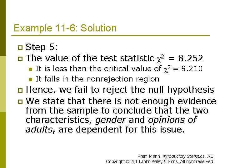
Example 11 -6: Solution Step 5: p The value of the test statistic χ2 = 8. 252 p n n It is less than the critical value of χ2 = 9. 210 It falls in the nonrejection region Hence, we fail to reject the null hypothesis p We state that there is not enough evidence from the sample to conclude that the two characteristics, gender and opinions of adults, are dependent for this issue. p Prem Mann, Introductory Statistics, 7/E Copyright © 2010 John Wiley & Sons. All right reserved

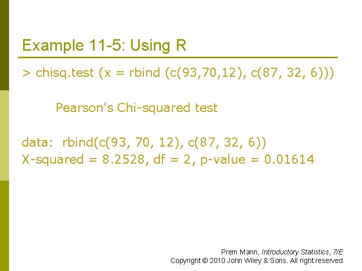
Example 11 -5: Using R > chisq. test (x = rbind (c(93, 70, 12), c(87, 32, 6))) Pearson's Chi-squared test data: rbind(c(93, 70, 12), c(87, 32, 6)) X-squared = 8. 2528, df = 2, p-value = 0. 01614 Prem Mann, Introductory Statistics, 7/E Copyright © 2010 John Wiley & Sons. All right reserved

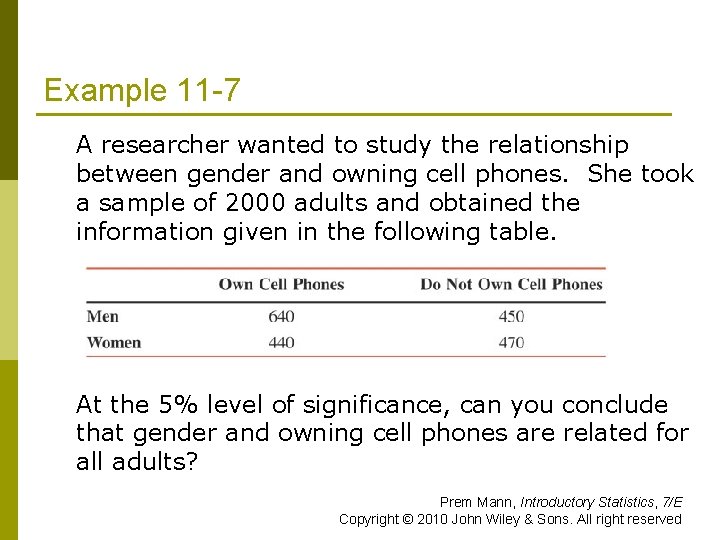
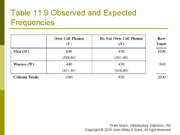
Example 11 -7 A researcher wanted to study the relationship between gender and owning cell phones. She took a sample of 2000 adults and obtained the information given in the following table. At the 5% level of significance, can you conclude that gender and owning cell phones are related for all adults? Prem Mann, Introductory Statistics, 7/E Copyright © 2010 John Wiley & Sons. All right reserved

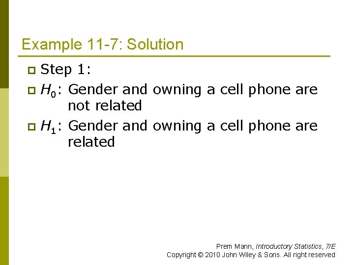
Example 11 -7: Solution Step 1: p H 0: Gender and owning a cell phone are not related p H 1: Gender and owning a cell phone are related p Prem Mann, Introductory Statistics, 7/E Copyright © 2010 John Wiley & Sons. All right reserved

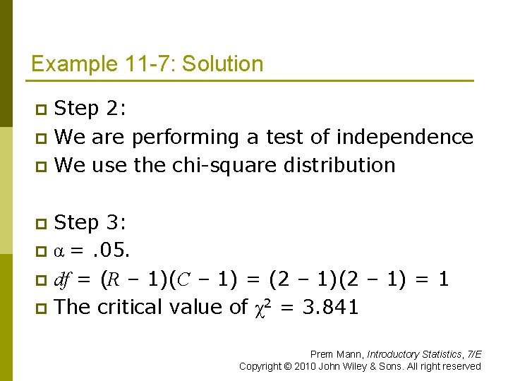
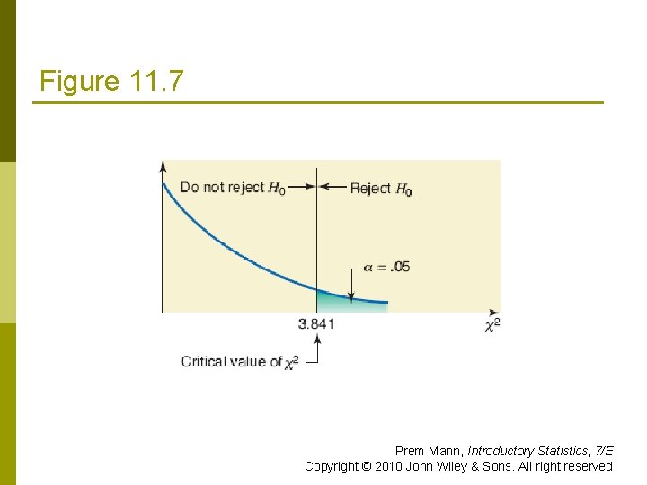
Example 11 -7: Solution Step 2: p We are performing a test of independence p We use the chi-square distribution p Step 3: p α =. 05. p df = (R – 1)(C – 1) = (2 – 1) = 1 p The critical value of χ2 = 3. 841 p Prem Mann, Introductory Statistics, 7/E Copyright © 2010 John Wiley & Sons. All right reserved

Figure 11. 7 Prem Mann, Introductory Statistics, 7/E Copyright © 2010 John Wiley & Sons. All right reserved

Table 11. 9 Observed and Expected Frequencies Prem Mann, Introductory Statistics, 7/E Copyright © 2010 John Wiley & Sons. All right reserved

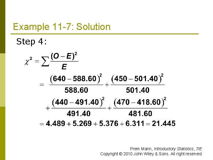
Example 11 -7: Solution Step 4: Prem Mann, Introductory Statistics, 7/E Copyright © 2010 John Wiley & Sons. All right reserved

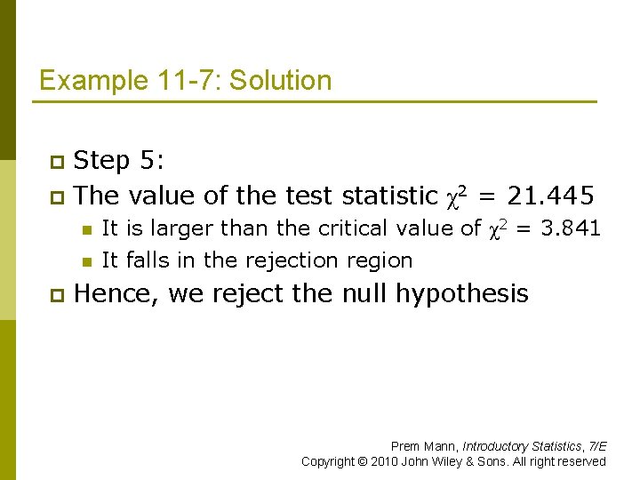
Example 11 -7: Solution Step 5: p The value of the test statistic χ2 = 21. 445 p n n p It is larger than the critical value of χ2 = 3. 841 It falls in the rejection region Hence, we reject the null hypothesis Prem Mann, Introductory Statistics, 7/E Copyright © 2010 John Wiley & Sons. All right reserved

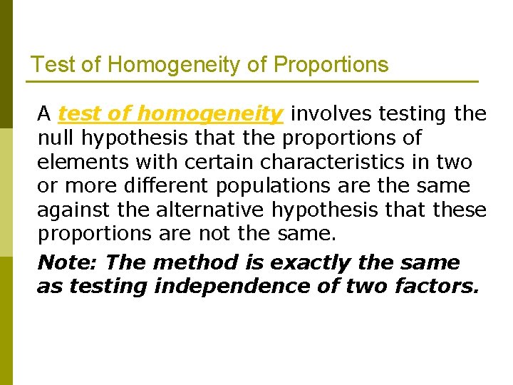
Test of Homogeneity of Proportions A test of homogeneity involves testing the null hypothesis that the proportions of elements with certain characteristics in two or more different populations are the same against the alternative hypothesis that these proportions are not the same. Note: The method is exactly the same as testing independence of two factors.

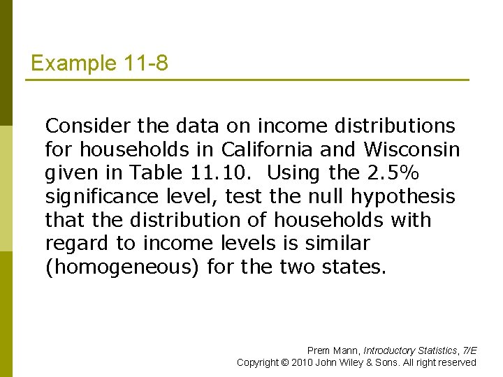
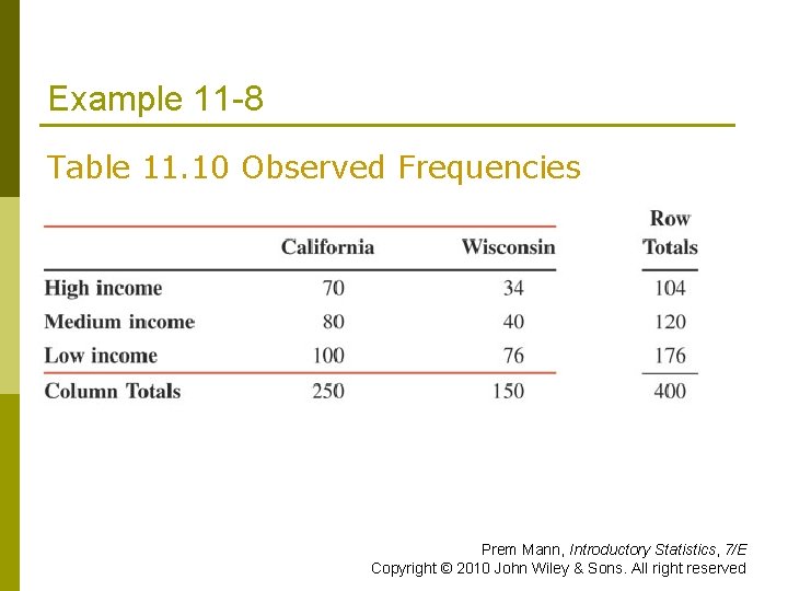
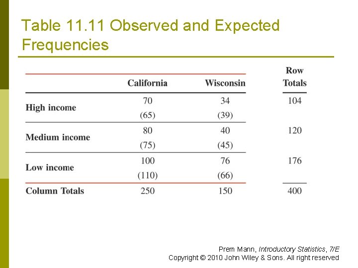
Example 11 -8 Consider the data on income distributions for households in California and Wisconsin given in Table 11. 10. Using the 2. 5% significance level, test the null hypothesis that the distribution of households with regard to income levels is similar (homogeneous) for the two states. Prem Mann, Introductory Statistics, 7/E Copyright © 2010 John Wiley & Sons. All right reserved

Example 11 -8 Table 11. 10 Observed Frequencies Prem Mann, Introductory Statistics, 7/E Copyright © 2010 John Wiley & Sons. All right reserved

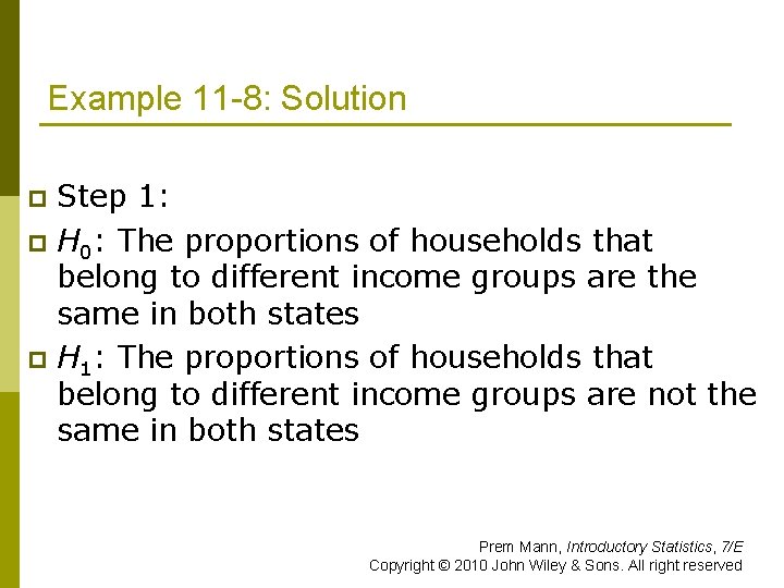
Example 11 -8: Solution Step 1: p H 0: The proportions of households that belong to different income groups are the same in both states p H 1: The proportions of households that belong to different income groups are not the same in both states p Prem Mann, Introductory Statistics, 7/E Copyright © 2010 John Wiley & Sons. All right reserved

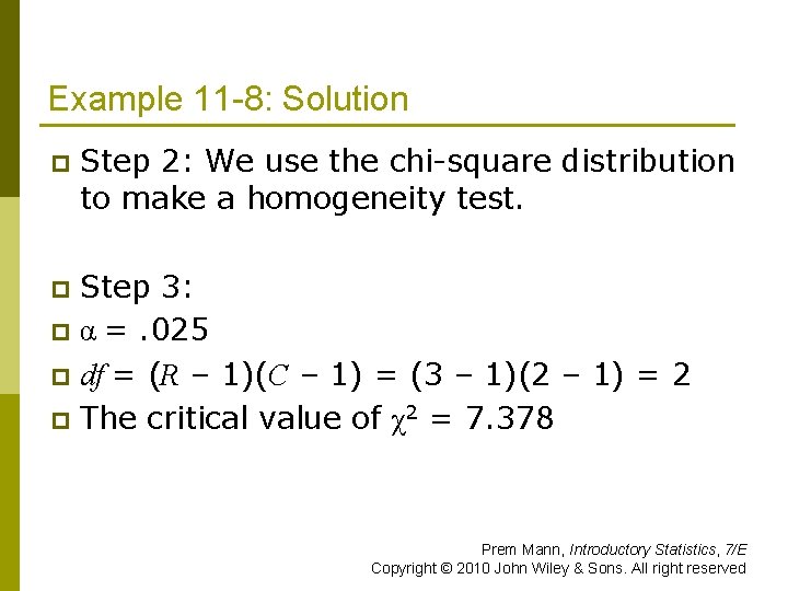
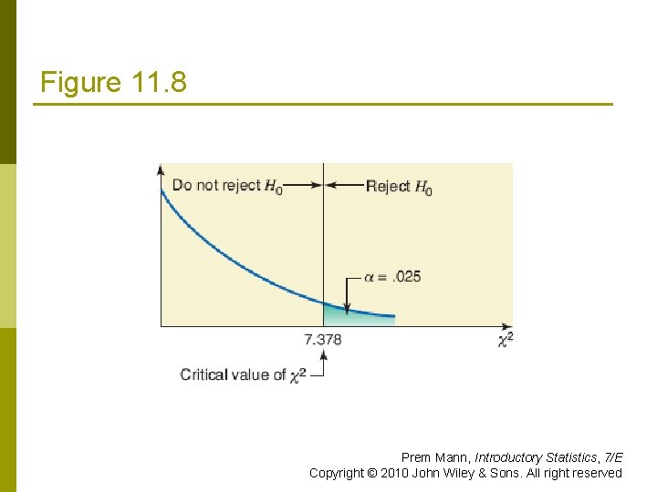
Example 11 -8: Solution p Step 2: We use the chi-square distribution to make a homogeneity test. Step 3: p α =. 025 p df = (R – 1)(C – 1) = (3 – 1)(2 – 1) = 2 p The critical value of χ2 = 7. 378 p Prem Mann, Introductory Statistics, 7/E Copyright © 2010 John Wiley & Sons. All right reserved

Figure 11. 8 Prem Mann, Introductory Statistics, 7/E Copyright © 2010 John Wiley & Sons. All right reserved

Table 11. 11 Observed and Expected Frequencies Prem Mann, Introductory Statistics, 7/E Copyright © 2010 John Wiley & Sons. All right reserved

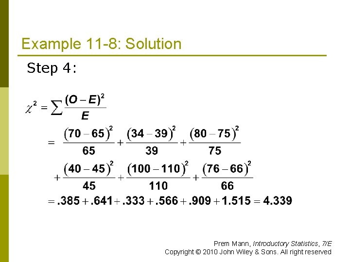
Example 11 -8: Solution Step 4: Prem Mann, Introductory Statistics, 7/E Copyright © 2010 John Wiley & Sons. All right reserved

Example 11 -8: Solution Step 5: p The value of the test statistic χ2 = 4. 339 p n n It is less than the critical value of χ2 It falls in the nonrejection region Hence, we fail to reject the null hypothesis p We state that the distribution of households with regard to income appears to be similar (homogeneous) in California and Wisconsin. p Prem Mann, Introductory Statistics, 7/E Copyright © 2010 John Wiley & Sons. All right reserved