CEE 320 Winter 2006 Trip Generation and Mode

CEE 320 Winter 2006 Trip Generation and Mode Choice CEE 320 Steve Muench

Outline 1. Trip Generation 2. Mode Choice CEE 320 Winter 2006 a. Survey

Trip Generation • Purpose – Predict how many trips will be made – Predict exactly when a trip will be made • Approach CEE 320 Winter 2006 – – Aggregate decision-making units Categorized trip types Aggregate trip times (e. g. , AM, PM, rush hour) Generate Model

Motivations for Making Trips • Lifestyle – – – Residential choice Work choice Recreational choice Kids, marriage Money CEE 320 Winter 2006 • Life stage • Technology

Reporting of Trips - Issues CEE 320 Winter 2006 • Under-reporting trivial trips • Trip chaining • Other reasons (passenger in a car for example)

Trip Generation Models • Linear (simple) CEE 320 Winter 2006 • Poisson (a bit better)

Poisson Distribution • Count distribution – Uses discrete values – Different than a continuous distribution P(n) = probability of exactly n trips being generated over time t n = number of trips generated over time t CEE 320 Winter 2006 λ = average number of trips over time, t t = duration of time over which trips are counted (1 day is typical)

Poisson Ideas • Probability of exactly 4 trips being generated – P(n=4) • Probability of less than 4 trips generated – P(n<4) = P(0) + P(1) + P(2) + P(3) • Probability of 4 or more trips generated – P(n≥ 4) = 1 – P(n<4) = 1 – (P(0) + P(1) + P(2) + P(3)) CEE 320 Winter 2006 • Amount of time between successive trips

Poisson Distribution Example Trip generation from my house is assumed Poisson distributed with an average trip generation per day of 2. 8 trips. What is the probability of the following: CEE 320 Winter 2006 1. Exactly 2 trips in a day? 2. Less than 2 trips in a day? 3. More than 2 trips in a day?

Example Calculations Exactly 2: Less than 2: CEE 320 Winter 2006 More than 2:

CEE 320 Winter 2006 Example Graph

CEE 320 Winter 2006 Example Graph

CEE 320 Winter 2006 Example: Time Between Trips

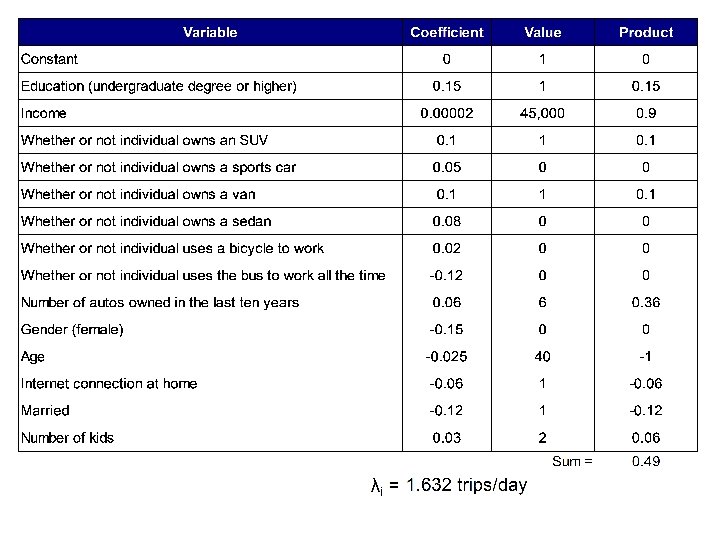
Example CEE 320 Winter 2006 Recreational or pleasure trips measured by λi (Poisson model):

Example • Probability of exactly “n” trips using the Poisson model: • Cumulative probability – Probability of one trip or less: – Probability of at least two trips: P(0) + P(1) = 0. 52 1 – (P(0) + P(1)) = 0. 48 • Confidence level CEE 320 Winter 2006 – We are 52% confident that no more than one recreational or pleasure trip will be made by the average individual in a day

Mode Choice • Purpose – Predict the mode of travel for each trip • Approach CEE 320 Winter 2006 – Categorized modes (SOV, HOV, bus, bike, etc. ) – Generate Model

CEE 320 Winter 2006 Qualitative Dependent Variable Dilemma Explanatory Variables

CEE 320 Winter 2006 Walk to School (yes/no variable) 1 = no, 0 = yes Dilemma = observation 1 0 0 Home to School Distance (miles) 10

A Mode Choice Model • Logit Model Specifiable part Unspecifiable part CEE 320 Winter 2006 • Final form s = all available alternatives m = alternative being considered n = traveler characteristic k = traveler

Discrete Choice Example CEE 320 Winter 2006 Regarding the TV sitcom Gilligan’s Island, whom do you prefer?

Ginger Model UGinger = 0. 0699728 – 0. 82331(carg) + 0. 90671(mang) + 0. 64341(pierceg) – 1. 08095(genxg) carg = Number of working vehicles in household mang = Male indicator (1 if male, 0 if female) pierceg = Pierce Brosnan indicator for question #11 (1 if Brosnan chosen, 0 if not) CEE 320 Winter 2006 genxg = generation X indicator (1 if respondent is part of generation X, 0 if not)

Mary Anne Model UMary Anne = 1. 83275 – 0. 11039(privatem) – 0. 0483453(agem) – 0. 85400(sinm) – 0. 16781(housem) + 0. 67812(seanm) + 0. 64508(collegem) – 0. 71374(llm) + 0. 65457(boomm) privatem = agem = sinm = housem = seanm = CEE 320 Winter 2006 collegem = number of years spent in a private school (K – 12) age in years single marital status indicator (1 if single, 0 if not) number of people in household Sean Connery indicator for question #11 (1 if Connery chosen, 0 if not) college education indicator (1 if college degree, 0 if not) llm = long & luxurious hair indicator for question #7 (1 if long, 0 if not) boomm = baby boom indicator (1 if respondent is a baby boomer, 0 if not)

No Preference Model Uno preference = – 9. 02430 x 10 -6(incn) – 0. 53362(gunsn) + 1. 13655(nojames) + 0. 66619(cafn) + 0. 96145(ohairn) incn = household income gunsn = gun ownership indicator (1 if any guns owned, 0 if no guns owned) nojames = No preference indicator for question #11 (1 if no preference, 0 if preference for a particular Bond) cafn = Caffeinated drink indicator for question #5 (1 if tea/coffee/soft drink, 0 if any other) CEE 320 Winter 2006 ohairn = Other hair style indicator for question #7 (1 if other style indicated, 0 if any style indicated)

CEE 320 Winter 2006 Results Average probabilities of selection for each choice are shown in yellow. These average percentages were converted to a hypothetical number of respondents out of a total of 207.

My Results Uginger = – 1. 1075 Umary anne = – 0. 2636 CEE 320 Winter 2006 Uno preference = – 0. 3265

CEE 320 Winter 2006 Primary References • Mannering, F. L. ; Kilareski, W. P. and Washburn, S. S. (2005). Principles of Highway Engineering and Traffic Analysis, Third Edition. Chapter 8 • Transportation Research Board. (2000). Highway Capacity Manual 2000. National Research Council, Washington, D. C.