Groundwater Pollution Remediation NOTE 2 Joonhong Park Yonsei

Groundwater Pollution Remediation (NOTE 2) Joonhong Park Yonsei CEE Department 2015. 10. 05. CEE 3330 Y 2013 WEEK 3

Darcy’s Experiment (1856) Flow of water in homogeneous sand filter under steady conditions A: cross area Sand Porous Medium h 2 L h 1 Datum Q = - K * A * (h 2 -h 1)/L CEE 3330 -01 May 8, 2007 Joonhong Park Copy K= hydraulic conductivity Right

Darcy’s Law Q = - K * A * (Φ 2 - Φ 1)/L Φ piezometric head In a 1 -D differential form, Darcy’s law may be: Darcy’s velocity: q = Q/A = d. V/[A*dt] = - K * [dΦ/d. L] Hydraulic Conductivity, K (L/T) KΞk*ρ*g/μ Here, k = intrinsic permeability (L 2) ρ: fluid density (M L-3); g: gravity (LT-2) μ: fluid dynamic viscosity (M L-1 T-1) CEE 3330 -01 May 8, 2007 Joonhong Park Copy Right

Modeling of Water Flow in Porous Media - Micro-scale modeling: the Navier-Stokes equation (flow through the void spaces in aquifers; fluid elements are described by differential equations ) - Macro-scale modeling: the Darcy’s equation (Darcy’s velocity: a volume flux defined as the volume of discharge per unit of bulk area) (What is seepage velocity? Velocity of a fluid element [v] vs Average v [q/n]) - Discussion (Differences? Advantages/Disadvantages? )

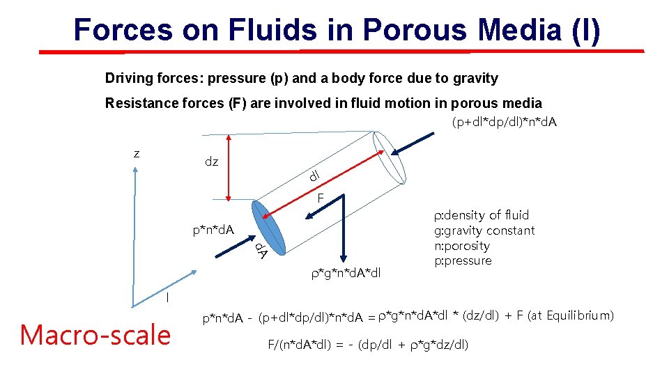
Forces on Fluids in Porous Media (I) Driving forces: pressure (p) and a body force due to gravity Resistance forces (F) are involved in fluid motion in porous media (p+dl*dp/dl)*n*d. A z dz dl F p*n*d. A ρ*g*n*d. A*dl ρ: density of fluid g: gravity constant n: porosity p: pressure l Macro-scale p*n*d. A - (p+dl*dp/dl)*n*d. A = ρ*g*n*d. A*dl * (dz/dl) + F (at Equilibrium) F/(n*d. A*dl) = - (dp/dl + ρ*g*dz/dl)

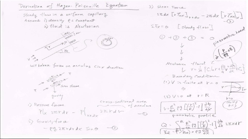
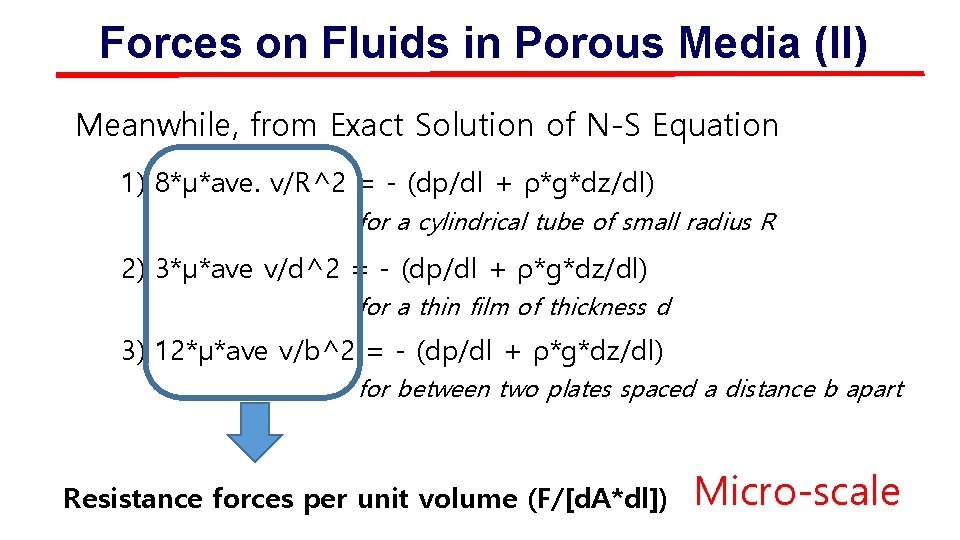
Forces on Fluids in Porous Media (II) Meanwhile, from Exact Solution of N-S Equation 1) 8*μ*ave. v/R^2 = - (dp/dl + ρ*g*dz/dl) for a cylindrical tube of small radius R 2) 3*μ*ave v/d^2 = - (dp/dl + ρ*g*dz/dl) for a thin film of thickness d 3) 12*μ*ave v/b^2 = - (dp/dl + ρ*g*dz/dl) for between two plates spaced a distance b apart Resistance forces per unit volume (F/[d. A*dl]) Micro-scale

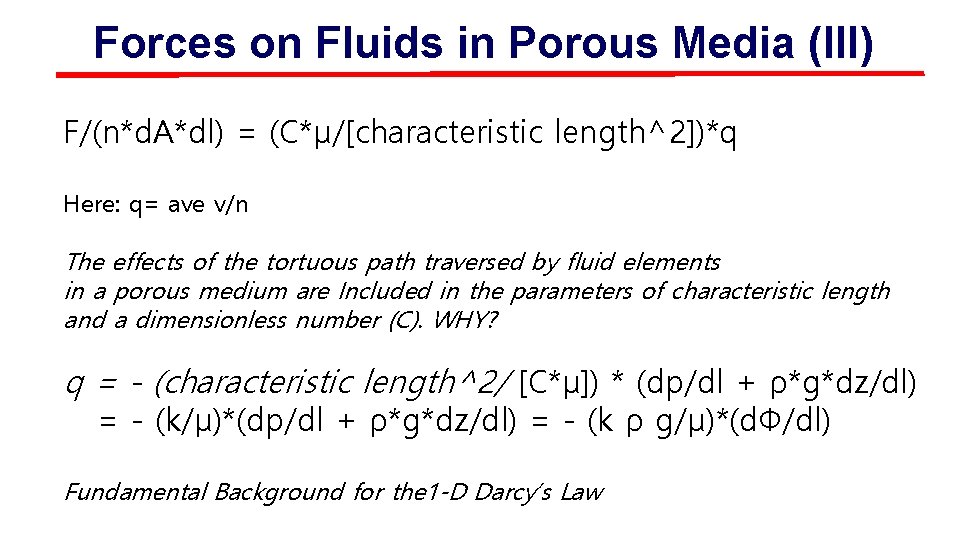
Forces on Fluids in Porous Media (III) F/(n*d. A*dl) = (C*μ/[characteristic length^2])*q Here: q= ave v/n The effects of the tortuous path traversed by fluid elements in a porous medium are Included in the parameters of characteristic length and a dimensionless number (C). WHY? q = - (characteristic length^2/ [C*μ]) * (dp/dl + ρ*g*dz/dl) = - (k/μ)*(dp/dl + ρ*g*dz/dl) = - (k ρ g/μ)*(d. Ф/dl) Fundamental Background for the 1 -D Darcy’s Law

Effect of turbulence q = - (k/μ)*(dp/dl + ρ*g*dz/dl) QUESTION: When can the linearity maintain or when cannot? (1) F/(n*d. A*dl) = (μ/k)*q + ρ*q^2/([k/C]^0. 5) = - (d. Ф/dl) (The Forchheimer’s equation) (q^2 is the inertial forces) (2) -([k/C]^0. 5/[ρ*q^2])*(d. Ф/dl) = μ/(ρ*q*([k*C]^0. 5) + 1 (3) f = 1/Re + 1 (f=the friction factor) when Re < 0. 02 [<0. 1], Darcy’s law is extremely exact [probably acceptable]

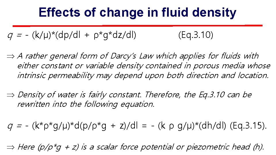
Effects of change in fluid density q = - (k/μ)*(dp/dl + ρ*g*dz/dl) (Eq. 3. 10) Þ A rather general form of Darcy’s Law which applies for fluids with either constant or variable density contained in porous media whose intrinsic permeability may depend upon both direction and location. Þ Density of water is fairly constant. Therefore, the Eq. 3. 10 can be rewritten into the following equation. q = - (k*ρ*g/μ)*d(p/ρ*g + z)/dl = - (k ρ g/μ)*(dh/dl) (Eq. 3. 15). Þ Here (p/ρ*g + z) is a scalar force potential or piezometric head (h).

3 -D Differential Form of Darcy’s Equation q = - (k ρ g/μ) * ∇h (Eq. 3. 17) ∇ = ∂/∂x * i + ∂/∂y * j + ∂/∂z * k (the gradient operator) Þ i, j, and k are the unit vectors in the x, y, and z coordinate directions, respectively. Þ Piezometric head is a scalar. Its negative gradient is a vector representing the force per unit weight acting on the fluid. (force potential) q = - (k ρ g/μ) * ∇h = -K * ∇h (Eq. 3. 20) Þ Barotropic fluids (ρ = function of p). However, constant density of water in most of groundwater is a good assumption. Of course, there are often exceptions. Þ Suppose K is constant (homogeneous). Then it is permissible to define Ф = K*h q = -∇ Ф (Eq. 3. 21)

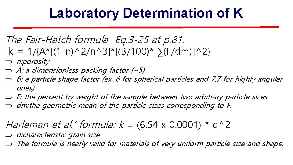
Laboratory Determination of K The Fair-Hatch formula Eq. 3 -25 at p. 81. k = 1/{A*[(1 -n)^2/n^3]*[(B/100)* ∑(F/dm)]^2} Þ n: porosity Þ A: a dimensionless packing factor (~5) Þ B: a particle shape factor (ex. 6 for spherical particles and 7. 7 for highly angular ones) Þ F: the percent by weight of the sample between two arbitrary particle sizes Þ dm: the geometric mean of the particle sizes corresponding to F. Harleman et al. ’ formula: k = (6. 54 x 0. 0001) * d^2 Þ d: characteristic grain size Þ The formula is nearly valid for materials of very uniform particle size and shape.

Carman-Kozeny Equation -k = Co * [n 3/(1 -n)2] * (1/SS 2) n: porosity SS: specific surface area or empirically, -k = [n 3/(1 -n)2] * (d. M 2/180) d. M: grain size for 50 percentile

Reading assignments Please read Darcy’s Law and the Equations of Groundwater Motion, p. 65 -82 including Example Example 3 -1 3 -2 3 -3 3 -4 3 -5 3 -6 3 -7

Non-Homogeneity Homogeneous: K is a scalar Heterotrophic: K is a function of positions at x, y, and z. K-a/K-b = tan (α-a) / tan (α-b) q-a α-a ∇ q-b K-b See p. 84 -87 α-b ∇ dl K-a

Anisotropy -∇h q-x q q-y

Reading assignments Please read Darcy’s Law and the Equations of Groundwater Motion, p. 82 -90 including - Flow parallel to the layers in a stratified aquifer - Flow through beds in series - Figure 3 -12 and Eq. 3. 39 to 3. 44 - See p. 70 -71 in the reading material

3 D Generalization of Darcy’s Law Heterotrophic Isotropic: q = - K (x, y, z) ∇ h ~ ~ For homogenous case, can rewrite as q= ~ - ∇ [K * h] = - ∇ Φ ~ ~ Anisotropic: q = - K ∇h = ~ ~ Kxx Kxy Kxz K= = Kyx Kyy Kyz Kzx Kzy Kzz

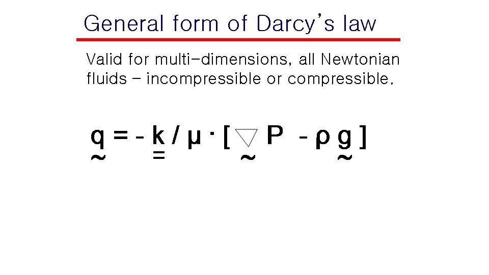
General form of Darcy’s law Valid for multi-dimensions, all Newtonian fluids – incompressible or compressible.

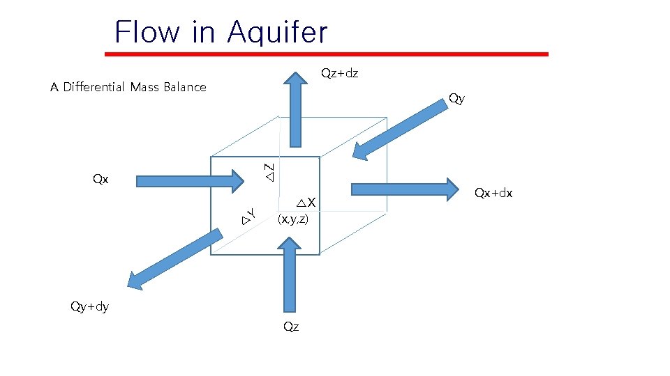
Flow in Aquifer Qz+dz A Differential Mass Balance △Z Qy Qx Y △ △X (x, y, z) Qy+dy Qz Qx+dx

Reading assignments Please read p. 58 -63 in the reading material - Governing Equation for Confined Aquifers Governing Equation for Unconfined Aquifers Governing Equation for Aquitards The Duipuit-Forchheimer Approximation The Boussinesq Equation Also read p. 72

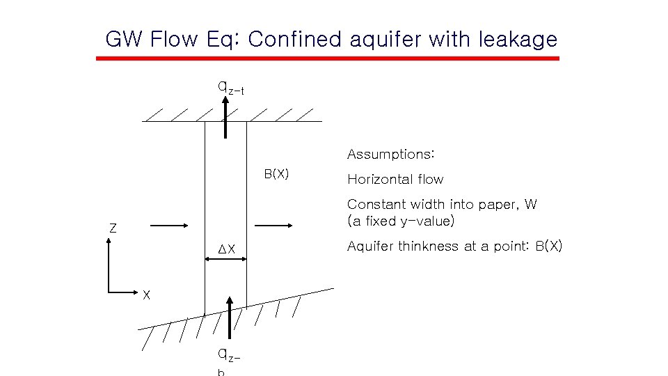
GW Flow Eq: Confined aquifer with leakage qz-t Assumptions: B(X) Horizontal flow Constant width into paper, W (a fixed y-value) Z ΔX X qz- Aquifer thinkness at a point: B(X)

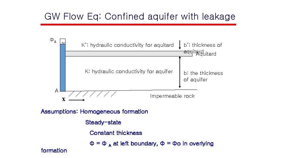
GW Flow Eq: Confined aquifer with leakage ФA K’: hydraulic conductivity for aquitard b’: thickness of aquitard Aquitard K: hydraulic conductivity for aquifer b: the thickness of aquifer A Impermeable rock x Assumptions: Homogeneous formation Steady-state Constant thickness Φ=Φ formation A at left boundary, Φ = Φo in overlying