Castro Neto A H The electronic properties of

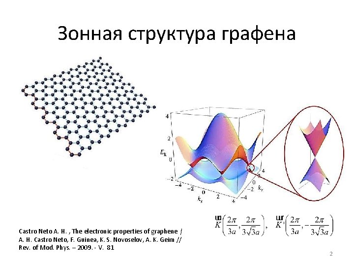
Зонная структура графена Castro Neto A. H. , The electronic properties of graphene | A. H. Castro Neto, F. Guinea, K. S. Novoselov, A. K. Geim // Rev. of Mod. Phys. – 2009. - V. 81 2

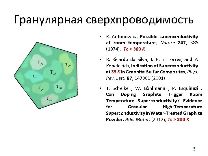
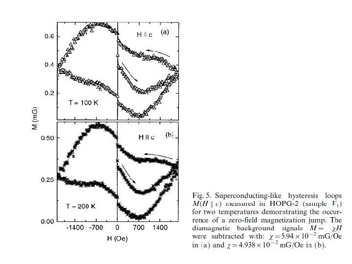
Гранулярная сверхпроводимость • K. Antonowicz, Possible superconductivity at room temperature, Nature 247, 385 (1974), Tc > 300 K • R. Ricardo da Silva, J. H. S. Torres, and Y. Kopelevich, Indication of Superconductivity at 35 K in Graphite-Sulfur Composites, Phys. Rev. Lett. 87, 147001 (2001) • T. Scheike , W. Böhlmann , P. Esquinazi , Can Doping Graphite Trigger Room Temperature Superconductivity? Evidence for Granular High-Temperature Superconductivity in Water-Treated Graphite Powder, Adv. Mater. (2012), Tc > 300 K 3

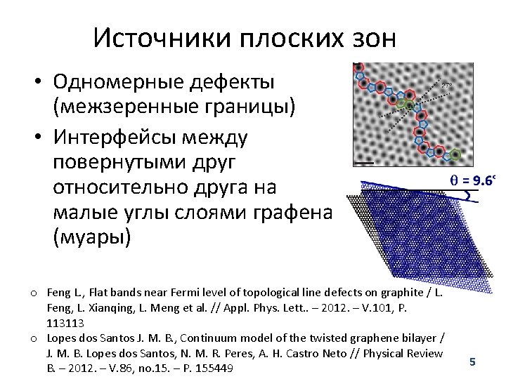
Источники плоских зон • Одномерные дефекты (межзеренные границы) • Интерфейсы между повернутыми друг относительно друга на малые углы слоями графена (муары) o Feng L. , Flat bands near Fermi level of topological line defects on graphite / L. Feng, L. Xianqing, L. Meng et al. // Appl. Phys. Lett. . – 2012. – V. 101, P. 113113 o Lopes dos Santos J. M. B. , Continuum model of the twisted graphene bilayer / J. M. B. Lopes dos Santos, N. M. R. Peres, A. H. Castro Neto // Physical Review B. – 2012. – V. 86, no. 15. – P. 155449 5

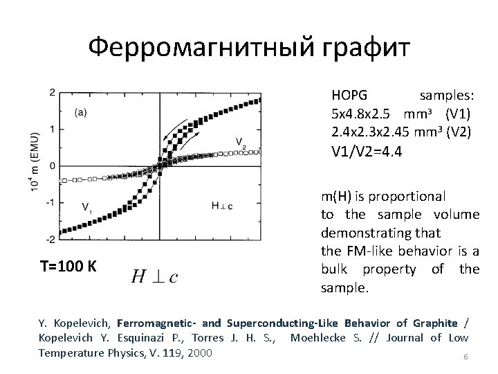
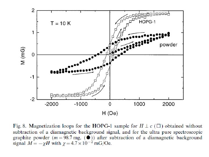
Ферромагнитный графит HOPG samples: 5 x 4. 8 x 2. 5 mm 3 (V 1) 2. 4 x 2. 3 x 2. 45 mm 3 (V 2) V 1/V 2=4. 4 T=100 K m(H) is proportional to the sample volume demonstrating that the FM-like behavior is a bulk property of the sample. Y. Kopelevich, Ferromagnetic- and Superconducting-Like Behavior of Graphite / Kopelevich Y. Esquinazi P. , Torres J. H. S. , Moehlecke S. // Journal of Low Temperature Physics, V. 119, 2000 6

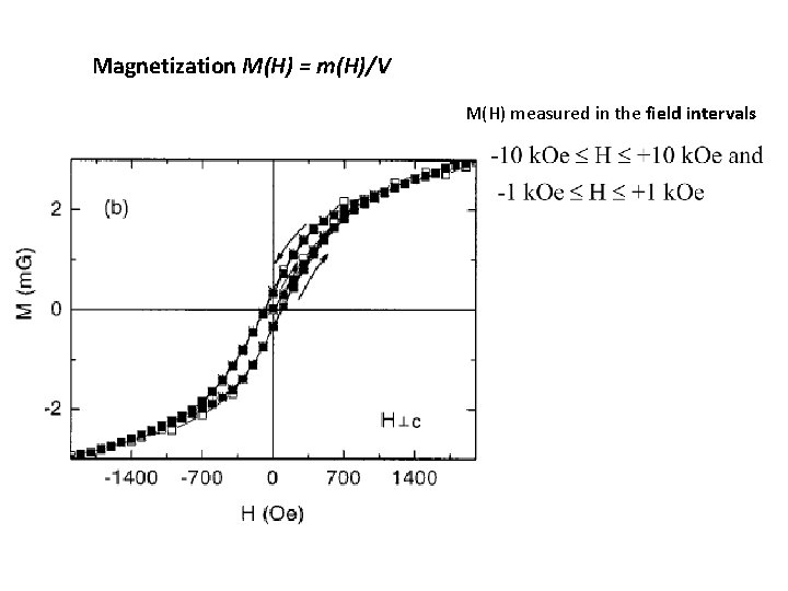
Magnetization M(H) = m(H)/V M(H) measured in the field intervals

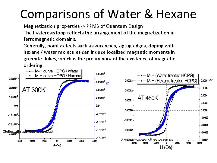
Comparisons of Water & Hexane Magnetization properties -> PPMS of Quantum Design The hysteresis loop reflects the arrangement of the magnetization in ferromagnetic domains. Generally, point defects such as vacancies, zigzag edges, doping with hexane / water molecules can induce localized magnetic moments in graphite flakes, which is the preliminary of the existence of magnetic ordering.

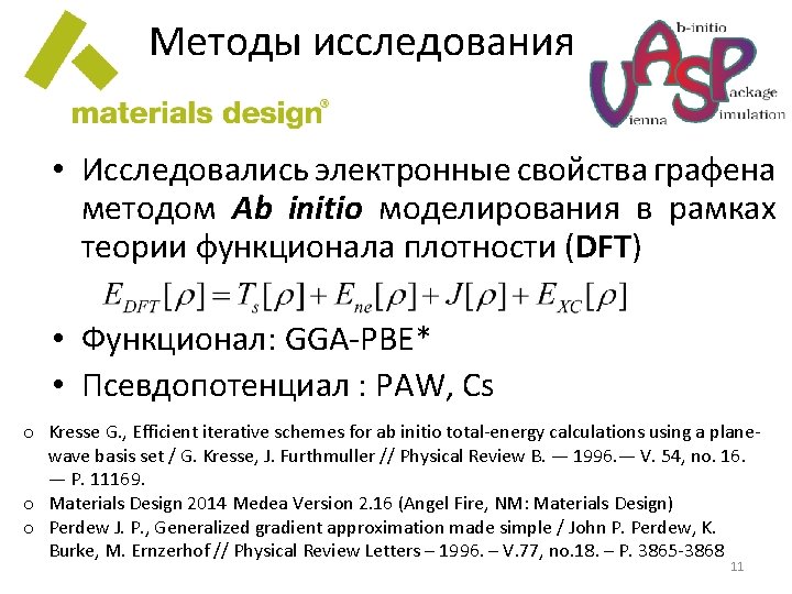
Методы исследования • Исследовались электронные свойства графена методом Ab initio моделирования в рамках теории функционала плотности (DFT) • Функционал: GGA-PBE* • Псевдопотенциал : PAW, Cs o Kresse G. , Efficient iterative schemes for ab initio total-energy calculations using a planewave basis set / G. Kresse, J. Furthmuller // Physical Review B. — 1996. — V. 54, no. 16. — P. 11169. o Materials Design 2014 Medea Version 2. 16 (Angel Fire, NM: Materials Design) o Perdew J. P. , Generalized gradient approximation made simple / John P. Perdew, K. Burke, M. Ernzerhof // Physical Review Letters – 1996. – V. 77, no. 18. – P. 3865 -3868 11

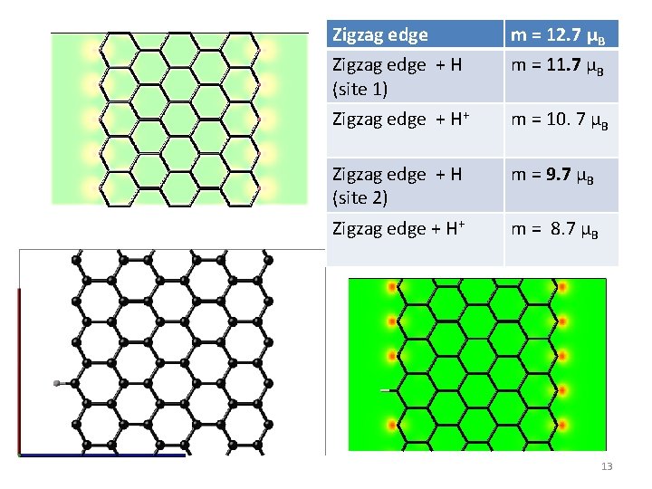
Zigzag edge m = 12. 7 μB Zigzag edge + H (site 1) m = 11. 7 μB Zigzag edge + H+ m = 10. 7 μB Zigzag edge + H (site 2) m = 9. 7 μB Zigzag edge + H+ m = 8. 7 μB 13

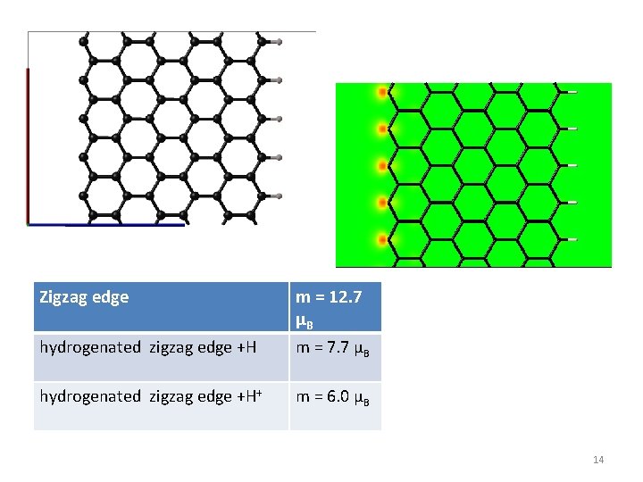
Zigzag edge hydrogenated zigzag edge +H m = 12. 7 μB m = 7. 7 μB hydrogenated zigzag edge +H+ m = 6. 0 μB 14

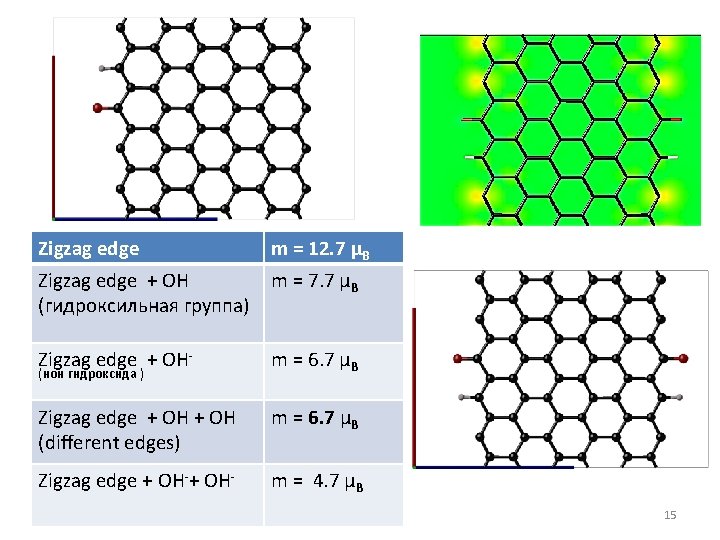
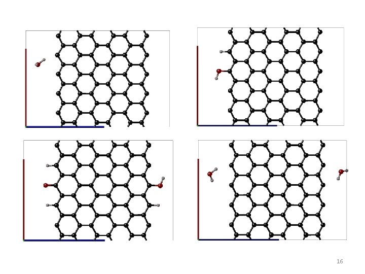
Zigzag edge m = 12. 7 μB Zigzag edge + OH (гидроксильная группа) m = 7. 7 μB Zigzag edge + OH- m = 6. 7 μB Zigzag edge + OH (different edges) m = 6. 7 μB Zigzag edge + OH- m = 4. 7 μB (ион гидроксида ) 15

16

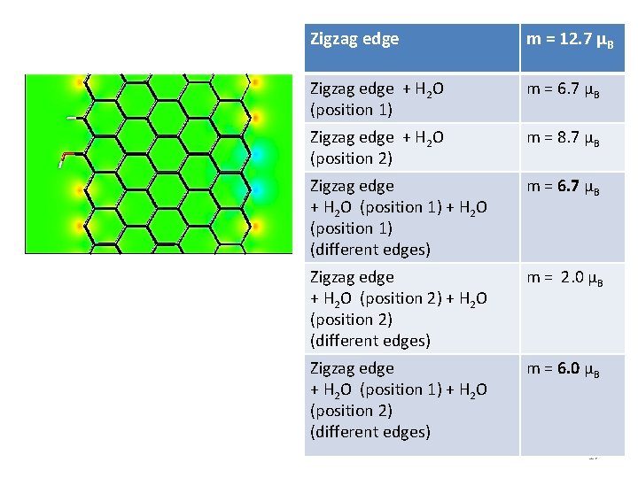
Zigzag edge m = 12. 7 μB Zigzag edge + H 2 O (position 1) m = 6. 7 μB Zigzag edge + H 2 O (position 2) m = 8. 7 μB Zigzag edge + H 2 O (position 1) + H 2 O (position 1) (different edges) m = 6. 7 μB Zigzag edge + H 2 O (position 2) + H 2 O (position 2) (different edges) m = 2. 0 μB Zigzag edge + H 2 O (position 1) + H 2 O (position 2) (different edges) m = 6. 0 μB 17

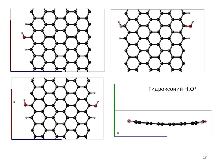
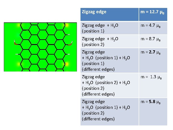
Zigzag edge m = 12. 7 μB Zigzag edge + H 3 O (position 1) m = 4. 7 μB Zigzag edge + H 2 O (position 2) m = 8. 7 μB Zigzag edge + H 3 O (position 1) + H 3 O (position 1) (different edges) m = 2. 7 μB Zigzag edge + H 3 O (position 2) + H 3 O (position 2) (different edges) m = 1. 3 μB Zigzag edge + H 3 O (position 1) + H 3 O (position 2) (different edges) m = 5. 8 μB 19

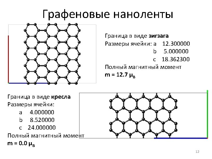
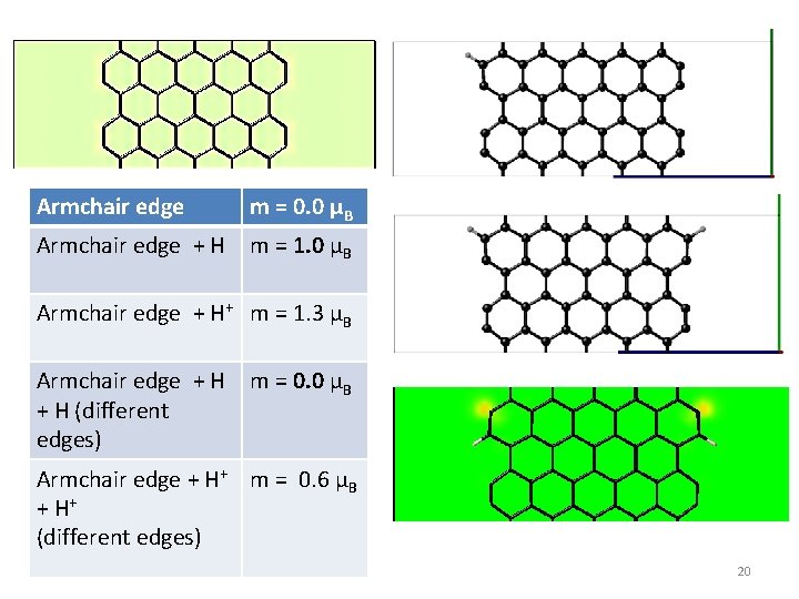
Armchair edge m = 0. 0 μB Armchair edge + H m = 1. 0 μB Armchair edge + H+ m = 1. 3 μB Armchair edge + H m = 0. 0 μB + H (different edges) Armchair edge + H+ m = 0. 6 μB + H+ (different edges) 20

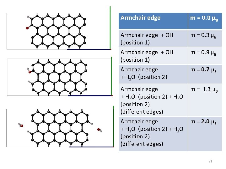
Armchair edge m = 0. 0 μB Armchair edge + OH (position 1) m = 0. 3 μB Armchair edge + OH- (position 1) m = 0. 9 μB Armchair edge + H 2 O (position 2) m = 0. 7 μB Armchair edge m = 1. 3 μB + H 2 O (position 2) + H 2 O (position 2) (different edges) Armchair edge m = 2. 0 μB + H 3 O (position 2) + H 3 O (position 2) (different edges) 21

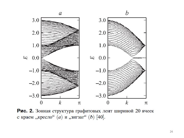
24

M-H curve in pure Bulk (a), and when after ultrasonicated in diluted hexane • RT (a) (b)