Calculus I Math 104 The end is near

Calculus I – Math 104 The end is near!

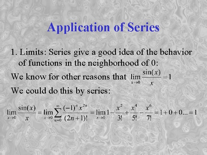
Application of Series 1. Limits: Series give a good idea of the behavior of functions in the neighborhood of 0: We know for other reasons that We could do this by series:

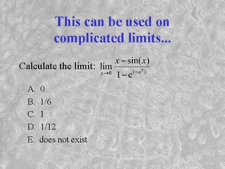
This can be used on complicated limits. . . Calculate the limit: A. B. C. D. E. 0 1/6 1 1/12 does not exist

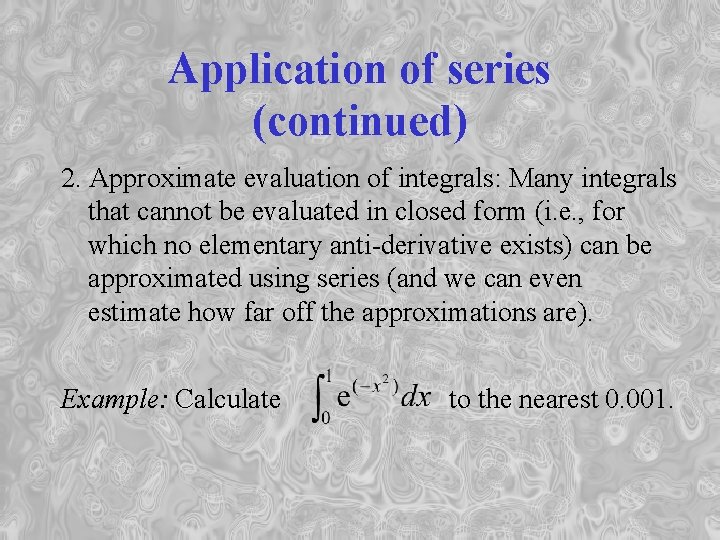
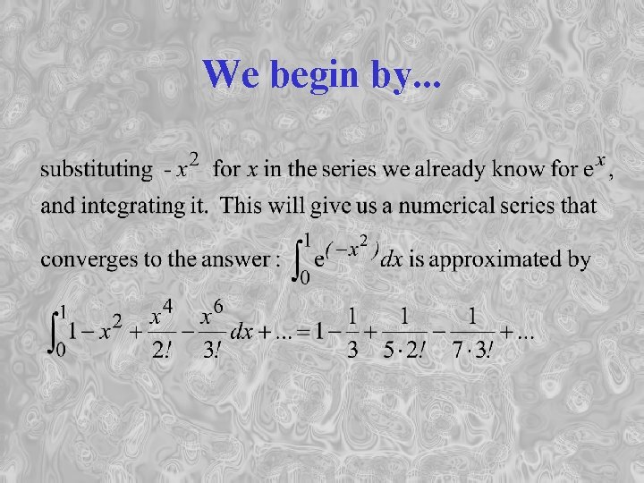
Application of series (continued) 2. Approximate evaluation of integrals: Many integrals that cannot be evaluated in closed form (i. e. , for which no elementary anti-derivative exists) can be approximated using series (and we can even estimate how far off the approximations are). Example: Calculate to the nearest 0. 001.

We begin by. . .

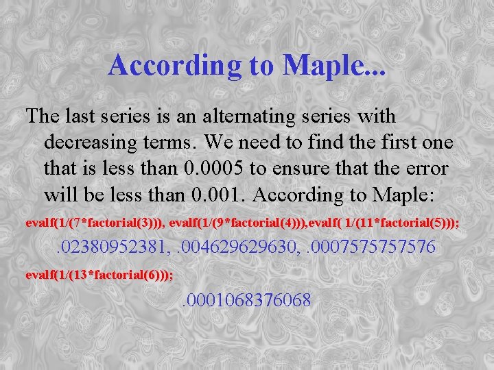
According to Maple. . . The last series is an alternating series with decreasing terms. We need to find the first one that is less than 0. 0005 to ensure that the error will be less than 0. 001. According to Maple: evalf(1/(7*factorial(3))), evalf(1/(9*factorial(4))), evalf( 1/(11*factorial(5))); . 02380952381, . 004629629630, . 000757576 evalf(1/(13*factorial(6))); . 0001068376068

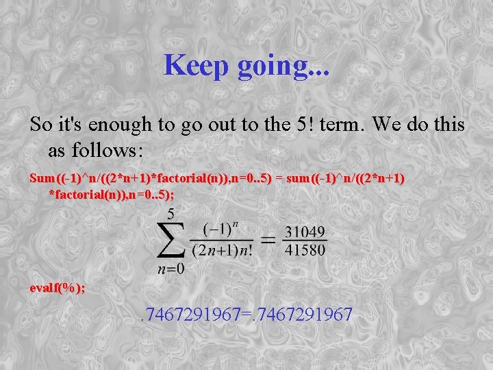
Keep going. . . So it's enough to go out to the 5! term. We do this as follows: Sum((-1)^n/((2*n+1)*factorial(n)), n=0. . 5) = sum((-1)^n/((2*n+1) *factorial(n)), n=0. . 5); evalf(%); . 7467291967=. 7467291967

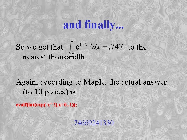
and finally. . . So we get that nearest thousandth. to the Again, according to Maple, the actual answer (to 10 places) is evalf(int(exp(-x^2), x=0. . 1)); . 74669241330

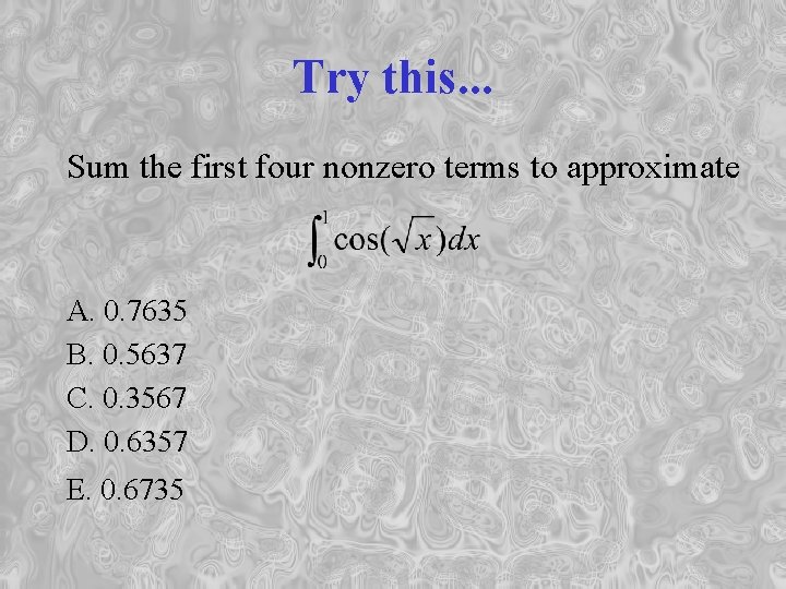
Try this. . . Sum the first four nonzero terms to approximate A. 0. 7635 B. 0. 5637 C. 0. 3567 D. 0. 6357 E. 0. 6735

Series approximations for functions, integrals etc. . We've been associating series with functions and using them to evaluate limits, integrals and such. We have not thought too much about how good the approximations are. For serious applications, it is important to do that.

Questions you can ask-1. If I use only the first three terms of the series, how big is the error? 2. How many terms do I need to get the error smaller than 0. 0001?

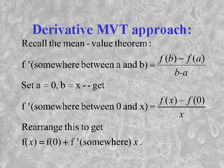
To get error estimates: Use a generalization of the Mean Value Theorem for derivatives

Derivative MVT approach:

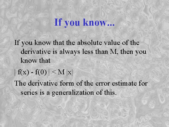
If you know. . . If you know that the absolute value of the derivative is always less than M, then you know that | f(x) - f(0) | < M |x| The derivative form of the error estimate for series is a generalization of this.

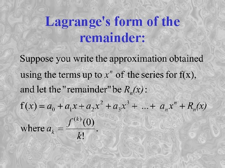
Lagrange's form of the remainder:

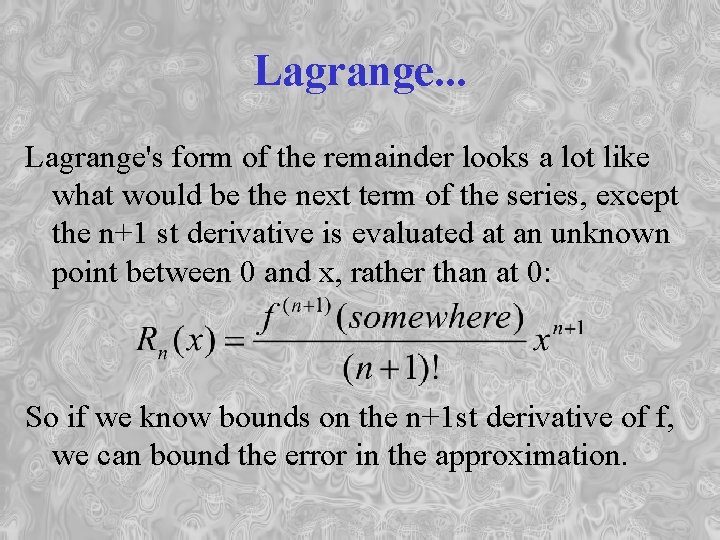
Lagrange. . . Lagrange's form of the remainder looks a lot like what would be the next term of the series, except the n+1 st derivative is evaluated at an unknown point between 0 and x, rather than at 0: So if we know bounds on the n+1 st derivative of f, we can bound the error in the approximation.

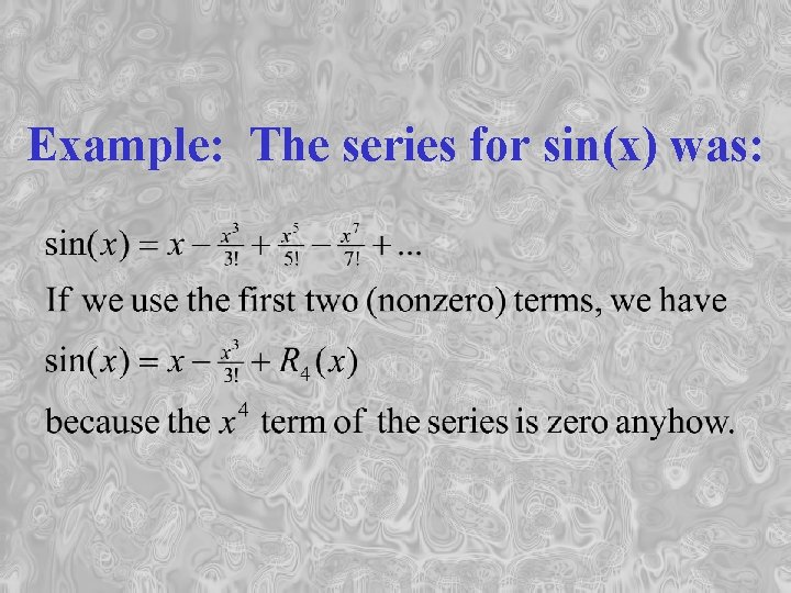
Example: The series for sin(x) was:

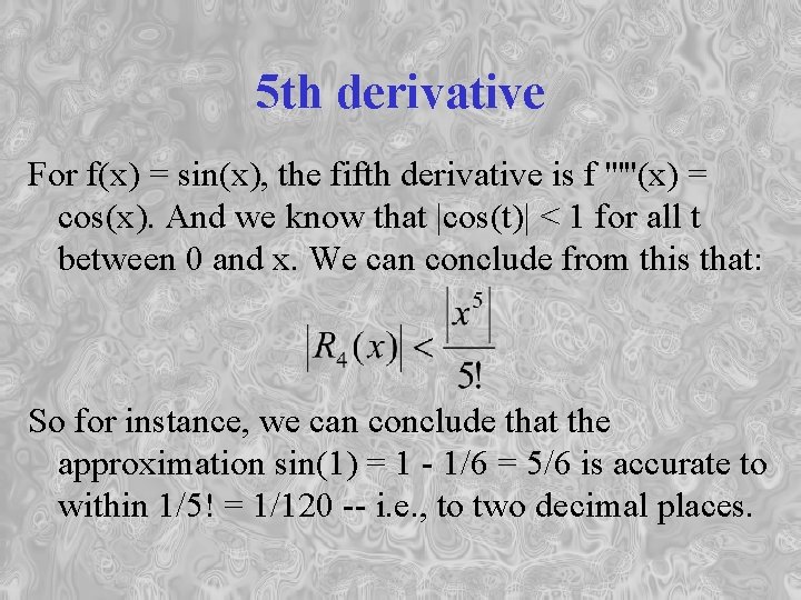
5 th derivative For f(x) = sin(x), the fifth derivative is f '''''(x) = cos(x). And we know that |cos(t)| < 1 for all t between 0 and x. We can conclude from this that: So for instance, we can conclude that the approximation sin(1) = 1 - 1/6 = 5/6 is accurate to within 1/5! = 1/120 -- i. e. , to two decimal places.

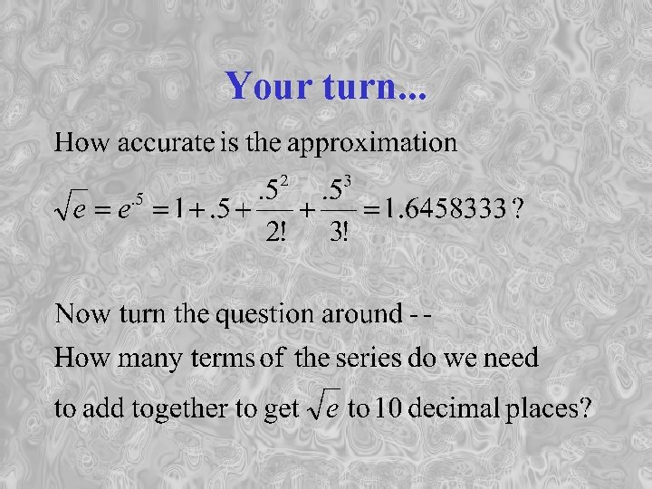
Your turn. . .

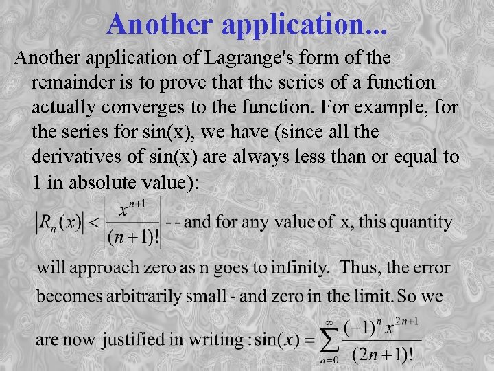
Another application. . . Another application of Lagrange's form of the remainder is to prove that the series of a function actually converges to the function. For example, for the series for sin(x), we have (since all the derivatives of sin(x) are always less than or equal to 1 in absolute value):

Shifting the origin -Taylor vs Maclaurin So far, we've been writing all of our series as infinite polynomials and using values of the function f(x) and its derivatives evaluated at x=0. It is possible to change one's point of view and use values of the function and derivatives at other points.

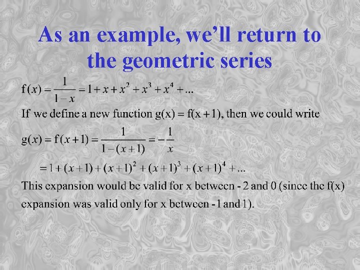
As an example, we’ll return to the geometric series

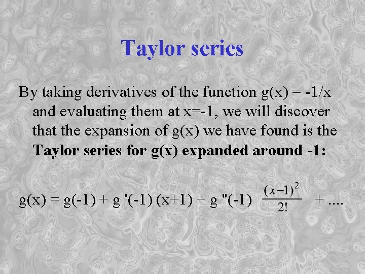
Taylor series By taking derivatives of the function g(x) = -1/x and evaluating them at x=-1, we will discover that the expansion of g(x) we have found is the Taylor series for g(x) expanded around -1: g(x) = g(-1) + g '(-1) (x+1) + g ''(-1) +. .

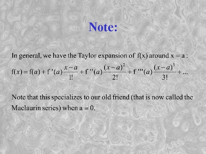
Note:

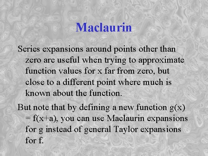
Maclaurin Series expansions around points other than zero are useful when trying to approximate function values for x far from zero, but close to a different point where much is known about the function. But note that by defining a new function g(x) = f(x+a), you can use Maclaurin expansions for g instead of general Taylor expansions for f.

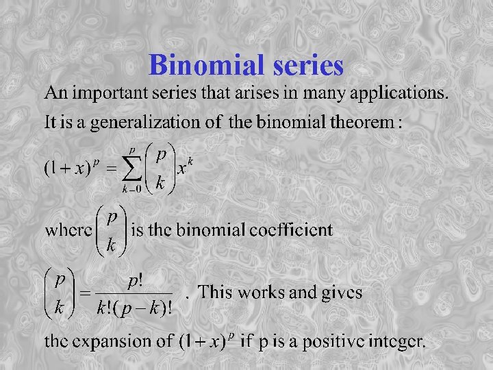
Binomial series

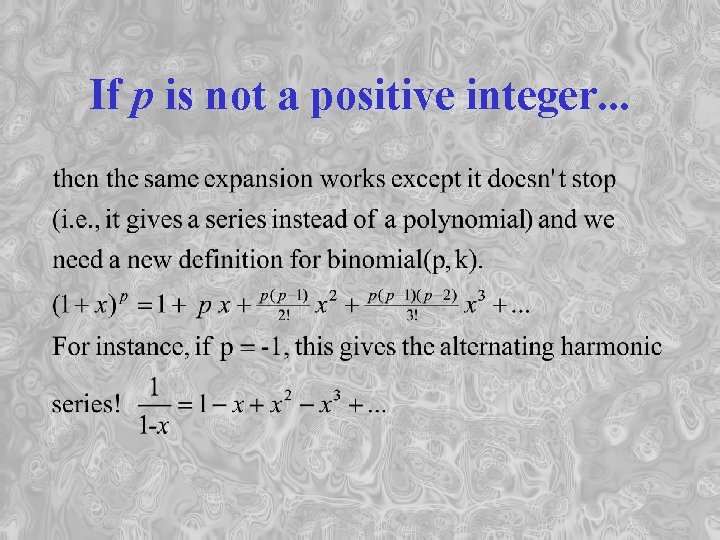
If p is not a positive integer. . .

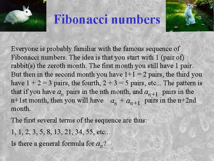
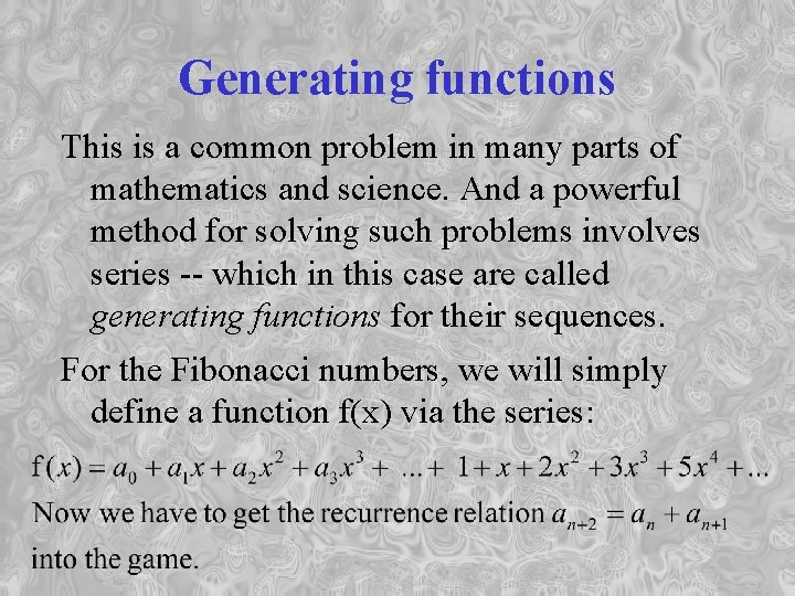
Fibonacci numbers Everyone is probably familiar with the famous sequence of Fibonacci numbers. The idea is that you start with 1 (pair of) rabbit(s) the zeroth month. The first month you still have 1 pair. But then in the second month you have 1+1 = 2 pairs, the third you have 1 + 2 = 3 pairs, the fourth, 2 + 3 = 5 pairs, etc. . . The pattern is that if you have an pairs in the nth month, and an+1 pairs in the n+1 st month, then you will have a n + a n+1 pairs in the n+2 nd month. The first several terms of the sequence are thus: 1, 1, 2, 3, 5, 8, 13, 21, 34, 55, etc. . . Is there a general formula for a n ?

Generating functions This is a common problem in many parts of mathematics and science. And a powerful method for solving such problems involves series -- which in this case are called generating functions for their sequences. For the Fibonacci numbers, we will simply define a function f(x) via the series:

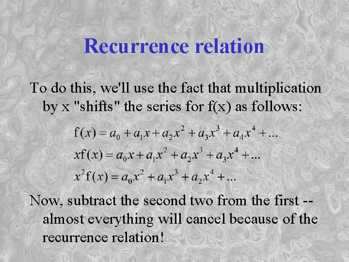
Recurrence relation To do this, we'll use the fact that multiplication by x "shifts" the series for f(x) as follows: Now, subtract the second two from the first -almost everything will cancel because of the recurrence relation!

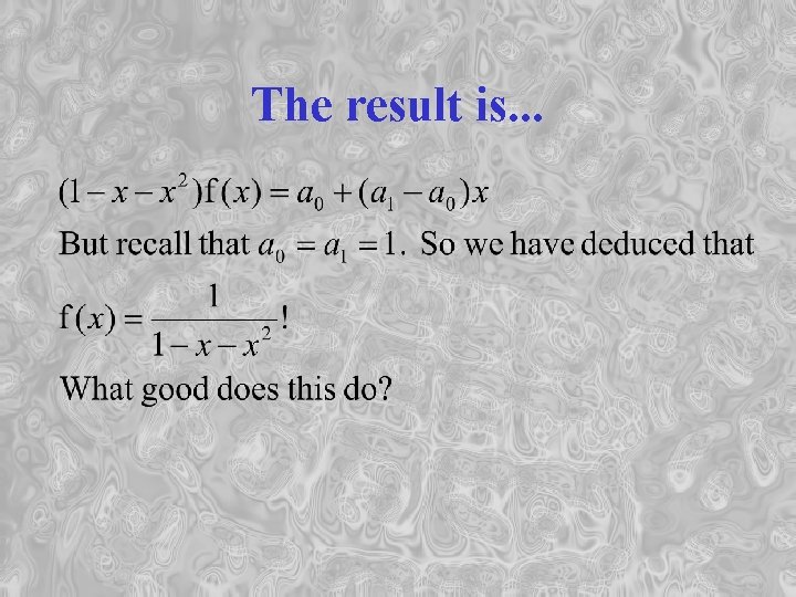
The result is. . .

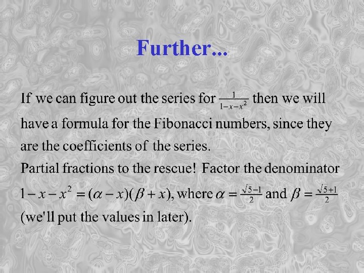
Further. . .

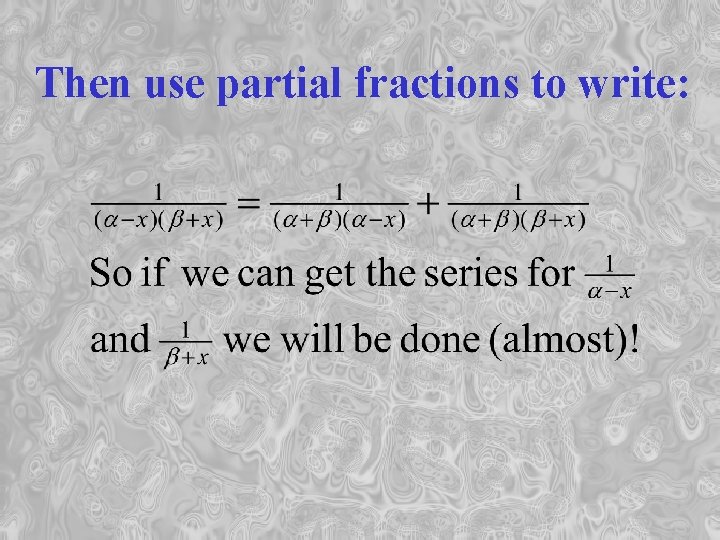
Then use partial fractions to write:

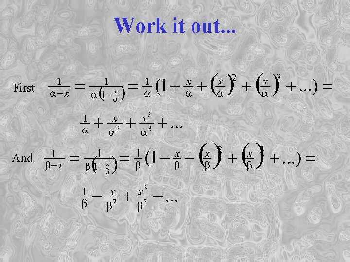
Work it out. . . First And

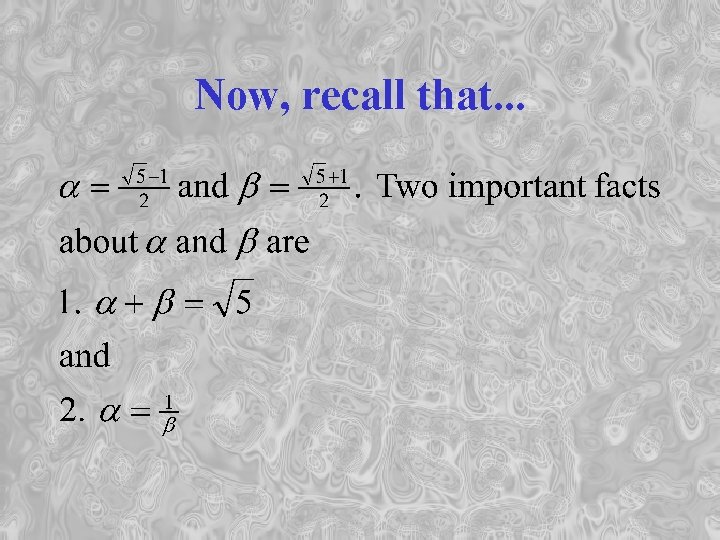
Now, recall that. . .

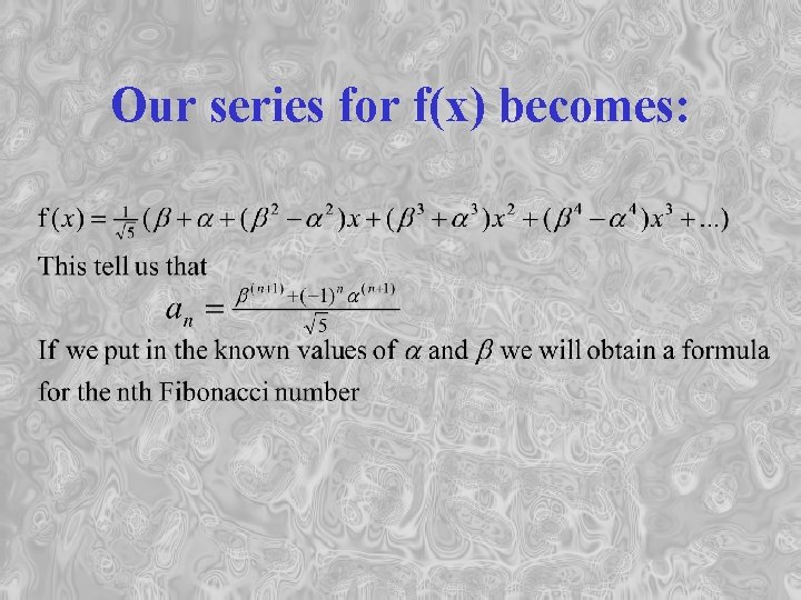
Our series for f(x) becomes: