Business Mathematics MTH367 Lecture 32 Chapter 20 Optimization

Business Mathematics MTH-367 Lecture 32

Chapter 20 Optimization: Functions of Several Variables continued

Last Lecture Summary We covered section 20. 2: Partial Derivatives Started Sec. 20. 3: Optimization of Bivariate Functions • Partial Derivatives of Bivariate Functions • Interpreting Partial Derivatives • Second-Order Partrial Derivatives

Today’s Topics We will continue with Sec. 20. 3: Optimization of Bivariate Functions • Review of Relative Extrema • Distinguishing Critical Points • Test for critical points • Applications of Bivariate Optimization

Optimization of Bivariate Functions We start with the revision of the optimization of bivariate functions, which was introduced in last lecture.
 is said to have a")
Revision • A function z = f (x, y) is said to have a relative maximum at x = a and y = b if for all points (x, y) “sufficiently close” to (a, b) f (a, b) ≥ f (x, y) • A function z = f (x, y) is said to have a relative minimum at x = a and y = b if for all points (x, y) “sufficiently close” (a, b) f (a, b) ≤ f (x, y)

Revision cont’d •


Distinguishing Nature of Critical Points • Once a critical point has been identified, it is necessary to determine its nature. • Aside from relative maximum and minimum points, there is one other situation in which fx and fy both equal 0. • Which is referred to as a saddle point. • A saddle point P is a portion of a surface which has the shape of a saddle. • At point P – “where you sit on the horse” – the value of fx and fy both equal 0. • However, the function does not reach either a relative maximum or a relative minimum at P.

Test of Critical Point Given that a critical point of f is located at (x*, y*, z) where all second partial derivatives are continuous, determine the value of D (x*, y*), where
>0, the critical point is a. b. A relative maximum if")
1. If D(x*, y*)>0, the critical point is a. b. A relative maximum if both fxx(x*, y*) and fyy(x*, y*) are negative. A relative minimum if both fxx(x*, y*) and fyy(x*, y*) are positive. 2. If D(x*, y*)<0, the critical point is a saddle point. 3. If D(x*, y*)=0, no conclusion.

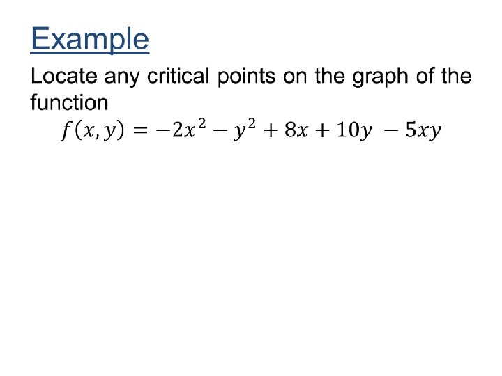
Example Given the function determine the location and nature of all critical points.


Applications of Bivariate Optimization This section presents some applications of the optimization of bivariate functions.
 is a function")
Example: Advertising Expenditures • A manufacturer’s estimated annual sales (in units) is a function of the expenditures made for radio and TV advertising. • The function specifying this relationship was stated as where z equals the number of units sold each year, x equals the amount spent for TV advertising and y equals the amount spent for radio advertising (x and y both in $1, 000 s).

Determine how much money should be spent on TV and radio advertising in order to sell maximum number of units.


Example: Pricing Model • A manufacturer sells two related products, the demands for which are estimated by the following two demand functions: where pj equals the price (in dollars) of product j and qj equals the demand (in thousands of units) for product j.

• Examination of these demand functions indicates that the two products are related. • The demand for one product depends not only on the price charged for the product itself but also on the price charged for the other product. • The firm wants to determine the price it should charge for each product in order to maximize total revenue from the sale of the two products.

Solution: • This revenue-maximizing problem is exactly like the single-product problems discussed in Chap. 17. • The only difference is that there are two products and two pricing decisions to be made. • Total revenue from selling the two products is determined by the function

• This function is stated in terms of four independent variables. • As with the single-product problems, we can substitute the right side of equations

We can now proceed to examine the revenue for relative maximum points. The first partial derivatives are


 is planning to")
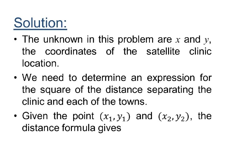
Example: Satellite Clinic Location • A large health maintenance organization (HMO) is planning to locate a satellite clinic in a location which is convenient to three suburban townships. • The relative locations of which are indicated in the Figure. • The HMO wants to select a preliminary site by using the following criterion: Determine the location (x, y) which minimize the sum of the squares of the distances from each township to the satellite clinic.

• Figure
")
• The square of the distance separating the clinic with location (x, y) and township A located at (40, 20) is • Similarly we can the formulae for townships B and C.

Finding similar expressions for the square of the distance separating township B and the clinic and summing for the three township, we get


Review We covered section 20. 3 and section 20. 4: : Optimization of Bivariate Functions • Critical Points and their types • Relative Maximum and Minimum • Test for critical points • Applications of Bivariate Optimization Finished the material for the course of Business Mathematics MTH-367.
- Slides: 36